
Hybrid search with BM25 and vector search
Hybrid search is a retrieval method that runs a keyword search and a vector search for the same query and merges the two ranked lists into one.
Last updated: 09 Oct, 2026 · rank-bm25 0.2.2
The retrieval tool of the agent in Agentic RAG API with FastAPI and LangGraph is a hybrid search over paper chunks. Keyword search finds the exact words of the question, which matters for names, ids and rare terms. Vector search finds text with the same meaning in different words. Each misses what the other finds, so the project runs both and fuses the results.
This part of the video starts at 6:40:36. It walks through the project's workflow documents for keyword search and hybrid search: BM25 for keywords, dense vectors for meaning, section-based chunking, 1024-dimension embeddings, metadata filters, and reciprocal rank fusion to combine the two result lists.
The project has no BM25 code of its own. Keyword search is the BM25 scoring built into OpenSearch, reached through a multi_match query, and the fusion is a search pipeline configured in OpenSearch; both are shown further down.
Two rankings and one fused list
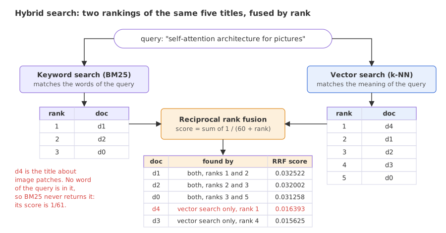
The picture is the result this lesson computes step by step on five paper titles: a BM25 ranking, a vector ranking, and the fused order. The titles are written from five papers in the project's paper table.
Scoring keywords with BM25
BM25 ("best match 25") scores a document for a query by adding one value per query term. It keeps the idea of TF-IDF, that a term counts more when it is frequent in the document and rare in the collection, and changes two things: repeated occurrences count less and less, and long documents are scaled down.
- idf, inverse document frequency, is large for a term few documents contain.
- k1 controls how fast repeated occurrences stop adding to the score.
- b controls how much a long document is penalised: 0 switches the length correction off, 1 applies it fully.
The example scores five titles for the query "transformer image" with the rank-bm25 library, then computes every score again from the formula.
import math

from rank_bm25 import BM25Okapi

corpus = ["Vector Policy Optimization trains policies for diverse rewards",        # d0
          "Attention is all you need introduces the transformer",                  # d1
          "Deep residual learning for image recognition",                          # d2
          "Balanced LoRA removes parameter invariance in low rank adaptation",     # d3
          "Transformer in transformer models image patches with a transformer"]    # d4
docs = [d.lower().split() for d in corpus]
query = "transformer image".split()

bm25 = BM25Okapi(docs)                       # k1 and b are read back below
library = bm25.get_scores(query)
N, avgdl, k1, b = len(docs), sum(len(d) for d in docs) / len(docs), bm25.k1, bm25.b
print(f"N = {N}  avgdl = {avgdl}  k1 = {k1}  b = {b}")

def idf(term, plus_one=False):               # n = documents that contain the term
    n = sum(term in d for d in docs)
    ratio = (N - n + 0.5) / (n + 0.5)
    return math.log(1 + ratio) if plus_one else math.log(ratio)

def score(doc, k1, b, plus_one=False):
    total = 0.0
    for term in query:
        tf = doc.count(term)
        total += idf(term, plus_one) * tf * (k1 + 1) / (tf + k1 * (1 - b + b * len(doc) / avgdl))
    return total

print("idf of each query term:", {t: round(idf(t), 4) for t in query})
print("doc  words  library  by hand  with ln(1 + ...) and k1 = 1.2")
for i, doc in enumerate(docs):
    print(f"d{i}   {len(doc):5}  {library[i]:7.4f}  {score(doc, k1, b):7.4f}  {score(doc, 1.2, 0.75, True):7.4f}")
print("order:", [f"d{i}" for i in sorted(range(N), key=lambda i: -library[i]) if library[i] > 0])N = 5 avgdl = 8.0 k1 = 1.5 b = 0.75
idf of each query term: {'transformer': 0.3365, 'image': 0.3365}
doc words library by hand with ln(1 + ...) and k1 = 1.2
d0 8 0.0000 0.0000 0.0000
d1 8 0.3365 0.3365 0.8755
d2 6 0.3791 0.3791 0.9752
d3 9 0.0000 0.0000 0.0000
d4 9 0.8623 0.8623 2.1727
order: ['d4', 'd2', 'd1']What the BM25 scores show
- The "by hand" column equals the library column on every row, so the formula above, with k1 = 1.5 and b = 0.75 read back from the object, is what
BM25Okapicomputes. - Both query terms have idf 0.3365: each occurs in two of the five titles.
- d4 is first with 0.8623. It holds "transformer" three times and "image" once.
- d2 (0.3791) is ahead of d1 (0.3365) although each holds one query term once. d2 has 6 words against an average of 8, and the length correction lifts short documents.
- The last column gives 2.1727, 0.9752 and 0.8755 for the same three titles. It uses an idf with 1 added inside the logarithm and k1 = 1.2, the idf form and the default of Lucene, the search library inside OpenSearch. The order is the same; the numbers are not. Lucene also leaves the constant factor k1 + 1 out of its score, so an engine's own numbers are smaller again, with the order unchanged.
- The idf without the 1 turns negative for a term that occurs in more than half of the documents;
rank-bm25then replaces it with a floor value, a fraction of the average idf. The form with the 1 never goes below zero.
Term-frequency saturation and length normalisation
The fraction in the formula is what separates BM25 from a raw word count. The plot draws it for the two k1 values above, and then for three values of b.
import matplotlib.pyplot as plt
import numpy as np

def tf_part(tf, k1, b=0.75, length_ratio=1.0):   # length_ratio = |d| / avgdl
    return tf * (k1 + 1) / (tf + k1 * (1 - b + b * length_ratio))

tf = np.arange(0, 21)
fig, (left, right) = plt.subplots(1, 2, figsize=(9, 3.6))
for k1 in (1.2, 1.5):
    left.plot(tf, tf_part(tf, k1), marker="o", markersize=3, label=f"k1 = {k1}")
    left.axhline(k1 + 1, linestyle="--", linewidth=0.8, color="gray")
left.plot(tf, tf, linestyle=":", color="black", label="raw count")
left.set_ylim(0, 3)
left.set_xticks(range(0, 21, 5))
left.set_xlabel("times the term appears in the document")
left.set_ylabel("term-frequency part of the score")
left.set_title("Saturation: the curve flattens below k1 + 1")
left.legend()

ratios = np.linspace(0.25, 4, 50)
for b in (0.0, 0.75, 1.0):
    right.plot(ratios, tf_part(1, 1.2, b, ratios), label=f"b = {b}")
right.set_xlabel("document length / average length")
right.set_title("Length normalisation at tf = 1, k1 = 1.2")
right.legend()
plt.tight_layout()
plt.show()

for k1 in (1.2, 1.5):
    print(f"k1 = {k1}:", [round(float(tf_part(t, k1)), 3) for t in (1, 2, 3, 5, 10, 100)], "limit", k1 + 1)
for b in (0.0, 0.75, 1.0):
    print(f"b = {b}:", [round(float(tf_part(1, 1.2, b, r)), 3) for r in (0.5, 1.0, 2.0)],
"for half, equal and double the average length")k1 = 1.2: [1.0, 1.375, 1.571, 1.774, 1.964, 2.174] limit 2.2 k1 = 1.5: [1.0, 1.429, 1.667, 1.923, 2.174, 2.463] limit 2.5 b = 0.0: [1.0, 1.0, 1.0] for half, equal and double the average length b = 0.75: [1.257, 1.0, 0.71] for half, equal and double the average length b = 1.0: [1.375, 1.0, 0.647] for half, equal and double the average length
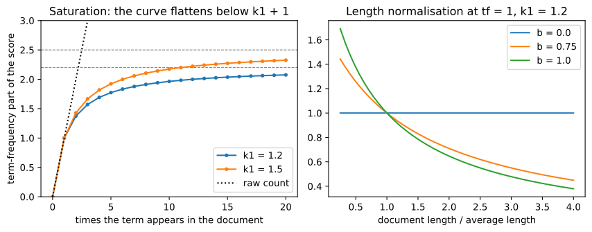
What the two panels show
- Repeats count less and less. With k1 = 1.2 one occurrence is worth 1.0, two 1.375, three 1.571, ten 1.964 and a hundred 2.174. The value can never pass k1 + 1 = 2.2. A raw count, the dotted line, would keep climbing.
- A larger k1 saturates more slowly. With k1 = 1.5, two, three and ten occurrences give 1.429, 1.667 and 2.174, under a ceiling of 2.5.
- b sets the length correction. At b = 0 a document of half, equal or double the average length gets 1.0 every time. At b = 0.75 the values are 1.257, 1.0 and 0.71, and at b = 1 they are 1.375, 1.0 and 0.647: the same single occurrence is worth less in a longer document.
Scoring meaning with embeddings
An embedding model turns a text into a vector, and texts with similar meaning get vectors that point in similar directions. Cosine similarity measures that: the dot product of two vectors divided by the product of their lengths. The query here is "self-attention architecture for pictures", which shares no content word with the title about image patches that it describes.
The project embeds with jina-embeddings-v3 at 1024 dimensions and lets OpenSearch run an approximate nearest-neighbour (k-NN) search over an HNSW index. The example below uses gemini-embedding-2 with a Gemini key, one text per call, and compares the query with every title in NumPy, which is exact and fast enough for five documents.
import os

import numpy as np
from google import genai

corpus = ["Vector Policy Optimization trains policies for diverse rewards",        # d0
          "Attention is all you need introduces the transformer",                  # d1
          "Deep residual learning for image recognition",                          # d2
          "Balanced LoRA removes parameter invariance in low rank adaptation",     # d3
          "Transformer in transformer models image patches with a transformer"]    # d4
query = "self-attention architecture for pictures"

client = genai.Client(api_key=os.environ["GEMINI_API_KEY"])

def embed(text):                             # one text per call
    reply = client.models.embed_content(model="gemini-embedding-2", contents=text)
    return np.array(reply.embeddings[0].values)

doc_vectors = np.array([embed(d) for d in corpus])
q = embed(query)
cosine = doc_vectors @ q / (np.linalg.norm(doc_vectors, axis=1) * np.linalg.norm(q))

print("vector length:", len(q))
for i in np.argsort(-cosine):
    print(f"d{i}  {cosine[i]:.4f}  {corpus[i]}")
print("dense order:", [f"d{i}" for i in np.argsort(-cosine)])vector length: 3072 d4 0.7599 Transformer in transformer models image patches with a transformer d1 0.7375 Attention is all you need introduces the transformer d2 0.6864 Deep residual learning for image recognition d3 0.6559 Balanced LoRA removes parameter invariance in low rank adaptation d0 0.5974 Vector Policy Optimization trains policies for diverse rewards dense order: ['d4', 'd1', 'd2', 'd3', 'd0']
What the cosine scores show
- Each vector has 3072 values.
- d4 is first with 0.7599. None of the content words of the query (self-attention, architecture, pictures) is in that title. The match is on meaning: "pictures" against "image patches", "self-attention architecture" against "transformer".
- d1, "Attention is all you need", is second with 0.7375.
- The scores sit between 0.5974 and 0.7599. Cosine similarities of unrelated short texts are not near zero, so the order and the gaps carry the information, not the absolute values.
Fusing two rankings with RRF
A BM25 score and a cosine similarity are on different scales, so they cannot be added as they are. Reciprocal rank fusion (RRF) ignores the scores and uses only the positions: each list gives a document 1 divided by a constant plus its rank, and the contributions are added.
The example ranks the same five titles for the same query with BM25, takes the dense order from the run above, and fuses them.
from rank_bm25 import BM25Okapi

corpus = ["Vector Policy Optimization trains policies for diverse rewards",        # d0
          "Attention is all you need introduces the transformer",                  # d1
          "Deep residual learning for image recognition",                          # d2
          "Balanced LoRA removes parameter invariance in low rank adaptation",     # d3
          "Transformer in transformer models image patches with a transformer"]    # d4
query = "self-attention architecture for pictures"

def tokens(text):
    return text.lower().replace("-", " ").split()

scores = BM25Okapi([tokens(d) for d in corpus]).get_scores(tokens(query))
keyword = [f"d{i}" for i in sorted(range(len(corpus)), key=lambda i: -scores[i]) if scores[i] > 0]
dense = ["d4", "d1", "d2", "d3", "d0"]       # the order the embedding run above printed

K = 60                                       # the rank constant
def rrf(doc):
    return sum(1 / (K + ranking.index(doc) + 1) for ranking in (keyword, dense) if doc in ranking)

print("keyword order:", keyword, "with BM25 scores", [round(float(s), 4) for s in scores])
print("dense order:  ", dense)
print("doc  keyword rank  dense rank  RRF score")
for doc in sorted(dense, key=rrf, reverse=True):
    k_rank = keyword.index(doc) + 1 if doc in keyword else "-"
    print(f"{doc}   {k_rank!s:>12}  {dense.index(doc) + 1:>10}  {rrf(doc):.6f}")
print("1/61 =", round(1 / 61, 6), "| 1/61 + 1/62 =", round(1 / 61 + 1 / 62, 6), "| 2/61 =", round(2 / 61, 6))keyword order: ['d1', 'd2', 'd0'] with BM25 scores [0.3365, 1.0986, 0.3791, 0.0, 0.0] dense order: ['d4', 'd1', 'd2', 'd3', 'd0'] doc keyword rank dense rank RRF score d1 1 2 0.032522 d2 2 3 0.032002 d0 3 5 0.031258 d4 - 1 0.016393 d3 - 4 0.015625 1/61 = 0.016393 | 1/61 + 1/62 = 0.032522 | 2/61 = 0.032787
What the fused order shows
- Keyword search returned three titles: d1, d2, d0. d1 matched "attention" (1.0986). d2 and d0 matched only the word "for" (0.3791 and 0.3365). d4 and d3 scored 0 and are not in the list.
- d1 is first with 0.032522, which is 1/61 + 1/62: rank 1 in one list and rank 2 in the other.
- d4, the best semantic match, is fourth with 0.016393 = 1/61. A document found by one search cannot pass a document found by both, whatever its rank: the most two lists can give is 2/61 = 0.032787.
- The word "for" decided third place. d0, the title on policy optimization, sits above d4 only because both it and the query contain "for". The project's index avoids this: its text analyzer lower-cases, removes stop words such as "for" and stems each word before anything is scored.
- Fusion inherits the weaknesses of both lists. RRF cannot tell a strong keyword match from a stop-word match; it sees only ranks.
The project's OpenSearch query
In the project one OpenSearch index, arxiv-papers-chunks, holds both the text of every chunk and its vector, so one request can run both searches. OpenSearch is a search engine with a k-NN plugin; no second vector store is involved.
The keyword part
return {
    "multi_match": {
        "query": self.query,
        "fields": self.fields,           # ["chunk_text^3", "title^2", "abstract^1"] for chunks
        "type": "best_fields",
        "operator": "or",
        "fuzziness": "AUTO",
        "prefix_length": 2,
    }
}
multi_match searches several fields at once. The ^3 and ^2 are boosts: a match in the chunk text counts three times, in the title twice. fuzziness: AUTO tolerates small typing errors. Each field is scored with the engine's BM25, whose settings in OpenSearch are k1 = 1.2 and b = 0.75 unless an index changes them.
The hybrid query
hybrid_query = {"hybrid": {"queries": [bm25_query, {"knn": {"embedding": {"vector": query_embedding, "k": size * 2}}}]}}

search_body = {
    "size": size,
    "query": hybrid_query,
    "_source": bm25_search_body["_source"],
    "highlight": bm25_search_body["highlight"],
}

response = self.client.search(
    index=self.index_name, body=search_body, params={"search_pipeline": HYBRID_RRF_PIPELINE["id"]}
)
A hybrid query holds sub-queries, here the keyword query and a knn query on the embedding field. Each sub-query asks for size * 2 candidates, so a request for three chunks fuses two lists of six.
The fusion pipeline
HYBRID_RRF_PIPELINE = {
    "id": "hybrid-rrf-pipeline",
    "description": "Post processor for hybrid RRF search",
    "phase_results_processors": [
        {
            "score-ranker-processor": {
                "combination": {
                    "technique": "rrf",  # Reciprocal Rank Fusion
                    "rank_constant": 60,  # Default k=60 for RRF formula: 1/(k+rank)
                }
            }
        }
    ],
}
Shown as it ran in the video, not run here: it needs an OpenSearch server, version 2.19 or later, with the index and its vectors. The score-ranker-processor with the rrf technique arrived in OpenSearch 2.19; a rank constant of 60 is also its default.
The trace in the video shows the pipeline at work: the top chunk of the answered request carries 'score': 0.016393442 and 'search_mode': 'hybrid'. That is 1/61, the value the example above printed for a document that is first in one list and absent from the other.
BM25 vs vector search vs hybrid search
| BM25 | Vector search | Hybrid with RRF | |
|---|---|---|---|
| Matches | The words of the query | The meaning of the query | Either |
| Strong on | Names, ids, rare terms, exact phrases | Paraphrases, synonyms, questions in other words | Mixed traffic |
| Misses | A document that uses different words | A rare exact term the model does not separate well | A document both searches rank low |
| Score | Unbounded, depends on the engine's formula | Cosine similarity, at most 1 | A sum of 1 / (60 + rank) |
| Needs | An inverted index | An embedding model and a vector index | Both, and a fusion step |
Where you use hybrid search
- RAG over technical text. Questions mix exact tokens (a paper id, a function name) with loose descriptions.
- Search with filters. The project's query filters by arXiv category before scoring, which matters more as the index grows.
- When you cannot tune weights. RRF has one constant and needs no score normalisation, so it is a safe first fusion method.
Related
- Previous: Amazon Bedrock Guardrails
- Next: Redis caching for RAG
- See also: Context precision
- Reference: OpenSearch: Score ranker processor, OpenSearch: Hybrid search, rank-bm25
- In the BM25 example, change the query to
"transformer transformer image": the query term is counted twice, d4 rises to 1.4061, and d1 (0.6729) moves ahead of d2. - In the RRF example, change
Kfrom 60 to 1 and read the order again: with a small constant, first place in one list is worth much more, and d4 moves up to third. - In the RRF example, remove the word
forfrom the query and run it: keyword search now returns d1 alone, and d4 is second in the fused list with 0.016393.
Every expert started right here.