
GRU (gated recurrent unit)
A GRU (gated recurrent unit) is a recurrent network cell that folds the LSTM's cell state into its hidden state and uses two gates, update and reset, to decide how much of the old state to keep and how much new information to write.
Last updated: 07 Oct, 2026 · TensorFlow 2 / Keras · NumPy
The LSTM (long short-term memory) has three gates and two states. Cho et al. (2014) proposed a lighter cell with the same goal, carrying information across many steps, using two gates and one state. With fewer weights it is cheaper to train, and on many sequence tasks it does about as well as an LSTM (Chung et al., 2014).
Reading the GRU equations
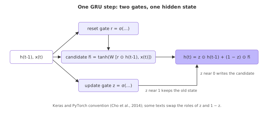
The GRU keeps only ht. Two sigmoid gates are computed from [ht−1, xt], as in the LSTM:
The reset gate decides how much of the old state the candidate sees. With r near 0 the candidate is computed almost from the current word alone, which lets the cell start fresh at a context switch:
The update gate then mixes the old state and the candidate, number by number:
This is the convention of Cho et al. and of the Keras and PyTorch code: z near 1 keeps the old state, z near 0 writes the candidate. Some texts, including Olah's LSTM post, swap z and 1 − z; the cell is the same, with the gate's meaning flipped.
Mapping the GRU gates to the LSTM gates
- The update gate does the work of the forget and input gates together. The LSTM keeps f ⊙ C and adds i ⊙ C̃ with two separate gates; the GRU keeps z ⊙ h and adds (1 − z) ⊙ h̃, so keeping more always means writing less.
- The reset gate has no LSTM twin. It controls how much of the old state goes into the candidate.
- There is no separate cell state and no output gate. The whole hidden state is passed on and shown as the output.
Running one GRU step in NumPy
The code runs one GRU step on the same sizes as the LSTM step, 4 inputs and 3 hidden units.
The update and reset gates
z = sigmoid(W_z @ np.concatenate([h_prev, x_t]))            # update gate
r = sigmoid(W_r @ np.concatenate([h_prev, x_t]))            # reset gate
The candidate and the new state
h_tilde = np.tanh(W_h @ np.concatenate([r * h_prev, x_t]))  # candidate state
h = z * h_prev + (1 - z) * h_tilde # keep (z) or replace (1 - z)import numpy as np
def sigmoid(z):
return 1 / (1 + np.exp(-z))
rng = np.random.default_rng(42)
D, H = 4, 3
x_t = rng.normal(0, 1, D) # the current word's vector
h_prev = rng.normal(0, 0.5, H) # h(t-1), the only state a GRU keeps
W_z, W_r, W_h = (rng.normal(0, 0.5, (H, H + D)) for _ in range(3))
z = sigmoid(W_z @ np.concatenate([h_prev, x_t])) # update gate
r = sigmoid(W_r @ np.concatenate([h_prev, x_t])) # reset gate
h_tilde = np.tanh(W_h @ np.concatenate([r * h_prev, x_t])) # candidate state
h = z * h_prev + (1 - z) * h_tilde # keep (z) or replace (1 - z)
for name, val in [("z", z), ("r", r), ("h~", h_tilde), ("h(t-1)", h_prev), ("h(t)", h)]:
print(f"{name:7s}", np.round(val, 4))
print("z = 1 keeps h(t-1):", np.allclose(1.0 * h_prev + 0.0 * h_tilde, h_prev))
print("GRU vs LSTM parameters, D=300, H=100:", 3 * (100 * (100 + 300) + 100), "vs", 4 * (100 * (100 + 300) + 100))
print("Keras GRU(100) on 40 numbers, reset_after=True:", 3 * 100 * (100 + 40) + 2 * 3 * 100)z [0.6027 0.3441 0.6032] r [0.4789 0.3846 0.5588] h~ [-0.5179 0.6832 0.2045] h(t-1) [-0.9755 -0.6511 0.0639] h(t) [-0.7937 0.2241 0.1197] z = 1 keeps h(t-1): True GRU vs LSTM parameters, D=300, H=100: 120300 vs 160400 Keras GRU(100) on 40 numbers, reset_after=True: 42600
What the GRU step shows
- h(t) sits between h(t−1) and h̃ on every unit, weighted by z: for the first unit 0.6027 × (−0.9755) + 0.3973 × (−0.5179) = −0.7937.
- z = 1 returns h(t−1) unchanged, the GRU's way of carrying memory forward. On that direct path the gradient back to h(t−1) is multiplied by z, which plays the role of the LSTM's forget gate.
- A GRU layer has three weight blocks to the LSTM's four: 120,300 against 160,400 parameters for D = 300 and H = 100.
- Keras counts 42,600 for GRU(100) on 40 inputs, because its default form keeps a second bias vector (see the Watch out below).
In Keras the layer is a drop-in swap for the LSTM:
from tensorflow.keras.layers import GRU

model.add(GRU(100))            # in place of model.add(LSTM(100))
GRU vs LSTM
| GRU | LSTM | |
|---|---|---|
| Gates | update z, reset r | forget f, input i, output o |
| States | ht only | ht and Ct |
| Keep vs write | tied: z and 1 − z | separate: f and i |
| Parameters, D = 300, H = 100 | 120,300 | 160,400 |
| Keras, 100 units on 40 inputs | 42,600 | 56,400 |
| Typical choice | smaller data, faster training | longer, more complex dependencies |
Where you use a GRU
- Text classification and tagging when an LSTM overfits or trains too slowly.
- On-device and streaming models, where fewer weights mean less memory and compute.
- Encoder-decoder models: the 2014 paper that introduced the GRU used it in a translation model.
reset_after=True, the default), a small variant of the equations above that adds a second bias vector. That is why GRU(100) on 40 inputs has 42,600 parameters, not 42,300, and weights saved from a model with reset_after=False do not load into the default layer.Related
- Previous: LSTM (long short-term memory)
- Next: Embedding layer in Keras
- Reference: Cho et al. (2014), Learning Phrase Representations using RNN Encoder-Decoder
- Set
rtonp.zeros(H)and compute h̃ again: the candidate now ignores h(t−1). - Replace the last line of the step with
h = (1 - z) * h_prev + z * h_tilde(the swapped convention) and compare h(t). - Compute the parameter count for D = 40, H = 100 with the formula 3 × (H × (H + D) + H) and compare it with Keras's 42,600.
Every expert started right here.