
Transformer encoder
The transformer encoder is a stack of identical layers that turns the embedded input tokens into contextual vectors; each layer runs multi-head self-attention and then a position-wise feed-forward network, each wrapped in a residual connection and layer normalization.
Last updated: 07 Oct, 2026 · NumPy
Self-attention, Multi-head attention, Positional encoding and Residual connections and layer normalization are the parts. The encoder is what you get when they are put together in the order the paper's figure draws them and repeated six times.
Following one encoder layer from input to output
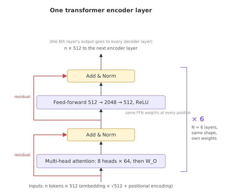
The research paper has six encoders and six decoders; for machine translation the input goes into the first encoder and the output comes out of the last decoder. Inside one encoder, the flow on the board runs bottom to top:
- Input sequence → text embeddings + positional encoding. Every word becomes a vector of 512 numbers, dmodel = 512 in the paper, and the positional encoding has the same size.
- Multi-head attention with 8 heads, Z1 to Z8. Each head works with query, key and value vectors of size 64 and divides its scores by √64 = 8.
- Add & Norm. The embedding + positional-encoding vectors skip around the attention and are added to its output (the residual), then layer normalization is applied.
- Feed-forward neural network, then a second Add & Norm, and the result goes to the next encoder.
In the paper the feed-forward network has a hidden layer of dff = 2048 units with ReLU between two linear layers, applied to each position separately with the same weights. Two details the board leaves out: the embeddings are multiplied by √dmodel before the positional encoding is added, and dropout of 0.1 is applied to each sub-layer's output before the residual add.
Stacking six encoder layers
Every layer takes an n × 512 matrix and returns an n × 512 matrix, so layers can be stacked. Each of the six has its own weights. The video's reason for many encoders is that sequence-to-sequence tasks such as translation are complex (one language, dialects, word order) and one encoder does not give good accuracy. Six is the paper's choice for its base model; its experiments also tried other depths. The output of the sixth encoder is the encoder's result: one contextual vector per input token, which every decoder layer reads through cross-attention.
Running a six-layer encoder in NumPy
Small sizes keep the printout readable: dmodel = 8, 2 heads of size 4, dff = 32, six layers, and three tokens for “Je suis étudiant”, the input of the video's encoder stack. The weights are random, so the numbers only show shapes and normalization, not meaning.
Sizes, layer norm and softmax
import numpy as np

d_model, h, d_ff, n_layers = 8, 2, 32, 6       # the paper uses 512, 8, 2048, 6
d_k = d_model // h

def layer_norm(x, eps=1e-5):
    mu = x.mean(axis=-1, keepdims=True)
    var = x.var(axis=-1, keepdims=True)
    return (x - mu) / np.sqrt(var + eps)        # gamma = 1, beta = 0

def softmax(s):
    e = np.exp(s - s.max(axis=-1, keepdims=True))
    return e / e.sum(axis=-1, keepdims=True)
Multi-head attention with the output projection
def multi_head(x, p):
    heads = []
    for i in range(h):
        Q, K, V = x @ p["WQ"][i], x @ p["WK"][i], x @ p["WV"][i]
        heads.append(softmax(Q @ K.T / np.sqrt(d_k)) @ V)
    return np.concatenate(heads, axis=-1) @ p["WO"]   # concat the heads, then W^O
The feed-forward network and one encoder layer
def ffn(x, p):
    return np.maximum(0, x @ p["W1"] + p["b1"]) @ p["W2"] + p["b2"]   # ReLU, per token

def encoder_layer(x, p):
    x = layer_norm(x + multi_head(x, p))        # sub-layer 1: attention, Add & Norm
    return layer_norm(x + ffn(x, p))            # sub-layer 2: feed-forward, Add & Norm
Random weights for one layer
def new_params():
    w = lambda *s: rng.normal(0, 0.3, s)
    return {"WQ": w(h, d_model, d_k), "WK": w(h, d_model, d_k), "WV": w(h, d_model, d_k),
            "WO": w(d_model, d_model), "W1": w(d_model, d_ff), "b1": np.zeros(d_ff),
"W2": w(d_ff, d_model), "b2": np.zeros(d_model)}rng = np.random.default_rng(42)
tokens = ["Je", "suis", "étudiant"]
x = rng.normal(0, 1, (len(tokens), d_model)) # embeddings + positional encoding
layers = [new_params() for _ in range(n_layers)] # six layers, each with its own weights
out = x
for i, p in enumerate(layers, start=1):
out = encoder_layer(out, p)
if i == 1:
print("after layer 1:", out.shape, " row means", np.round(out.mean(axis=1), 4) + 0.0,
" row stds", np.round(out.std(axis=1), 4))
print("after layer 6:", out.shape)
print("token 'suis' in, first 4 values: ", np.round(x[1, :4], 3))
print("token 'suis' out, first 4 values:", np.round(out[1, :4], 3))after layer 1: (3, 8) row means [0. 0. 0.] row stds [1. 1. 1.] after layer 6: (3, 8) token 'suis' in, first 4 values: [-0.017 -0.853 0.879 0.778] token 'suis' out, first 4 values: [ 0.516 -1.794 0.834 -0.455]
What the six layers produced
- The shape never changes: (3, 8) after layer 1 and after layer 6, one vector per token.
- Every row has mean 0 and standard deviation 1 after a layer, because the last step of each layer is a layer norm with γ = 1 and β = 0.
- The vector for “suis” changed from [−0.017, −0.853, 0.879, 0.778] to [0.516, −1.794, 0.834, −0.455] in its first four values: after attention it carries information from “Je” and “étudiant” too.
Counting the weights in the paper's encoder
d_model, h, d_ff, N = 512, 8, 2048, 6
d_k = d_model // h

mha = 4 * (d_model * d_model + d_model)           # W_Q, W_K, W_V, W_O with biases
ffn = d_model * d_ff + d_ff + d_ff * d_model + d_model
norms = 2 * (2 * d_model)                         # two layer norms, gamma and beta each
layer = mha + ffn + norms

print("d_k = d_model / h =", d_k)
print("multi-head attention:", f"{mha:,}")
print("feed-forward network:", f"{ffn:,}")
print("two layer norms:     ", f"{norms:,}")
print("one encoder layer:   ", f"{layer:,}")
print("six encoder layers: ", f"{N * layer:,}")d_k = d_model / h = 64 multi-head attention: 1,050,624 feed-forward network: 2,099,712 two layer norms: 2,048 one encoder layer: 3,152,384 six encoder layers: 18,914,304
- dk = 512 / 8 = 64, so the 8 heads together cost the same as one head of size 512.
- The feed-forward network holds two thirds of a layer's weights: 2,099,712 of 3,152,384.
- Six layers come to 18,914,304 weights, before the embeddings and the decoder.
Encoder layer vs decoder layer
| Encoder layer | Decoder layer | |
|---|---|---|
| Sub-layers | self-attention, feed-forward | masked self-attention, cross-attention, feed-forward |
| Add & Norm boxes | 2 | 3 |
| Sees | all input tokens at once | earlier output tokens and the whole encoder output |
| Mask | padding mask only | look-ahead + padding in self-attention; source padding in cross-attention |
| Runs at inference | once per input | once per generated token |
Where you use the transformer encoder
- Translation and summarization: the encoder half of an encoder-decoder model reads the source.
- BERT-style models: an encoder stack alone, for classification, named entities and search.
- Sentence embeddings: the encoder's output vectors, averaged or taken at a special token.
x + multi_head(x) fails with a shape error. The feed-forward hidden size is 2048 in the paper, but its output is back to 512.Related
- Previous: Residual connections and layer normalization
- Next: Masked self-attention
- See also: Transformer architecture
- Reference: Attention Is All You Need (Vaswani et al., 2017)
- Set
n_layers = 1and compare the output of “suis” with the six-layer run. - Change
h, d_ffto4, 16(so d_k = 2) and confirm the output shape stays (3, 8). - In the weight count, set
d_ff = 4 * d_modelfor d_model = 768 and compare with BERT-base's 3072.
This is what real progress feels like.