
Vanishing and exploding gradients in RNNs
Vanishing and exploding gradients are the two ways backpropagation through time fails on long sequences: the product of one factor per step shrinks towards zero or grows without bound, so the early words get almost no say in training, or the updates blow up.
Last updated: 07 Oct, 2026 · TensorFlow 2 / Keras · NumPy
Backpropagation through time (BPTT) ended with each step's term shrinking as it went back through the sentence. This lesson follows that product over a hundred steps and shows the opposite failure as well.
Shrinking gradients in a long RNN
The forward and backward passes repeat for a number of epochs, and training can stop early once the loss stops falling. The trouble starts with long sentences: the example had 4 time steps, but a long text has 100, 200 or 300. Unrolled, that is a very deep network.
Every step passes through an activation function. The sigmoid's output lies between 0 and 1 and its derivative between 0 and 0.25. Going back step after step multiplies such small numbers together, so the gradient gets smaller and smaller, the weight updates for the early steps become negligible, and the weights there barely change. This is the vanishing gradient problem, and the LSTM (long short-term memory) network was designed to ease it.
Most RNNs use tanh in the hidden state, whose derivative can reach 1, so the activation alone is not the whole story. Each step back multiplies by diag(1 − h²)·Wh, the derivative and the recurrent weights. When the size of that factor stays below 1 the product vanishes; above 1 it can explode.
import numpy as np
import matplotlib.pyplot as plt

z = np.linspace(-6, 6, 1201)
sig = 1 / (1 + np.exp(-z))
d_sig = sig * (1 - sig)                 # derivative of sigmoid
d_tanh = 1 - np.tanh(z) ** 2            # derivative of tanh
print("largest sigmoid derivative:", round(float(d_sig.max()), 4), "at z =", round(float(z[d_sig.argmax()]), 2))
print("largest tanh derivative:   ", round(float(d_tanh.max()), 4), "at z =", round(float(z[d_tanh.argmax()]), 2))
for k in (5, 10, 20, 50):
    print(f"0.25 multiplied {k} times: {0.25 ** k:.2e}")

plt.figure(figsize=(7, 3.6))
plt.plot(z, d_sig, label="sigmoid derivative (max 0.25)")
plt.plot(z, d_tanh, label="tanh derivative (max 1)")
plt.xlabel("z")
plt.title("Derivatives of sigmoid and tanh")
plt.legend(loc="upper right", fontsize=9)
plt.show()largest sigmoid derivative: 0.25 at z = 0.0 largest tanh derivative: 1.0 at z = 0.0 0.25 multiplied 5 times: 9.77e-04 0.25 multiplied 10 times: 9.54e-07 0.25 multiplied 20 times: 9.09e-13 0.25 multiplied 50 times: 7.89e-31
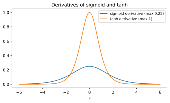
- The sigmoid derivative peaks at 0.25 and tanh's at 1, both at z = 0.
- 0.25 multiplied 10 times is 9.54 × 10⁻⁷, and 50 times is 7.89 × 10⁻³¹: ten sigmoid steps already cut a gradient a million-fold even at the best possible point.
Losing the context of early words
The video's next-word example: "On Sunday I want to eat pizza, on Monday I want to eat ___". The network reads the whole sentence and predicts one word at the end, so it is many to one. The right answer depends on "Sunday" and "Monday", which sit far back from the blank.
An RNN handles a sentence of four or five words well, because every word is close to the output. With a long sentence the output may depend on the first or second word, and the gradient from those early steps has been multiplied by many small factors before it arrives. An RNN therefore behaves like a short-term memory: recent words dominate, distant ones fade.
Measuring the gradient product over 100 steps
The code runs a 100-step tanh RNN and multiplies the factors ∂ht/∂ht−1 going back from the last step. It also multiplies Wh by itself for two scalings, 0.9 and 1.5, which is the product when every tanh derivative is 1.
Two recurrent matrices of known size
A random matrix is divided by its largest eigenvalue size, so 0.9·R and 1.5·R have largest eigenvalue sizes of exactly 0.9 and 1.5.
rng = np.random.default_rng(7)
H, D, T = 8, 4, 100
R = rng.normal(0, 1, (H, H))
R = R / np.abs(np.linalg.eigvals(R)).max()   # largest eigenvalue size scaled to 1
W_small, W_big = 0.9 * R, 1.5 * R            # two recurrent matrices
The product of the step factors
h, hs = np.zeros(H), []
for t in range(T):                           # a real 100-step tanh RNN with W_small
    h = np.tanh(W_x @ X[t] + W_small @ h)
    hs.append(h)
J = np.eye(H)
for k in range(1, T + 1):                    # dh_100 / dh_(100-k), one factor per step back
J = J @ (np.diag(1 - hs[T - k] ** 2) @ W_small)import numpy as np
import matplotlib.pyplot as plt
rng = np.random.default_rng(7)
H, D, T = 8, 4, 100
X = rng.normal(0, 1, (T, D))
W_x = rng.normal(0, 0.5, (H, D))
R = rng.normal(0, 1, (H, H))
R = R / np.abs(np.linalg.eigvals(R)).max() # largest eigenvalue size scaled to 1
W_small, W_big = 0.9 * R, 1.5 * R
h, hs = np.zeros(H), []
for t in range(T):
h = np.tanh(W_x @ X[t] + W_small @ h)
hs.append(h)
ks = np.arange(1, T + 1)
J, tanh_rnn = np.eye(H), []
for k in ks:
J = J @ (np.diag(1 - hs[T - k] ** 2) @ W_small)
tanh_rnn.append(np.linalg.norm(J, 2))
small = [np.linalg.norm(np.linalg.matrix_power(W_small, k), 2) for k in ks]
big = [np.linalg.norm(np.linalg.matrix_power(W_big, k), 2) for k in ks]
for k in (1, 10, 50, 100):
print(f"k={k:3d} tanh RNN {tanh_rnn[k - 1]:.1e} W_small^k {small[k - 1]:.1e} W_big^k {big[k - 1]:.1e}")
plt.figure(figsize=(7, 4))
plt.semilogy(ks, tanh_rnn, label="tanh RNN, W_h scaled to 0.9")
plt.semilogy(ks, small, "--", label="W_h^k, scaled to 0.9")
plt.semilogy(ks, big, label="W_h^k, scaled to 1.5")
plt.semilogy(ks, 0.25 ** ks, ":", label="0.25^k")
plt.ylim(1e-30, 1e30)
plt.xlabel("k, steps back from the last word")
plt.ylabel("size of the gradient factor")
plt.title("Gradient factors over 100 steps: vanish below 1, explode above 1")
plt.legend(loc="upper left")
plt.show()k= 1 tanh RNN 1.1e+00 W_small^k 1.3e+00 W_big^k 2.2e+00 k= 10 tanh RNN 1.3e-02 W_small^k 8.9e-01 W_big^k 1.5e+02 k= 50 tanh RNN 1.0e-12 W_small^k 1.8e-02 W_big^k 2.3e+09 k=100 tanh RNN 8.3e-24 W_small^k 9.5e-05 W_big^k 1.5e+18
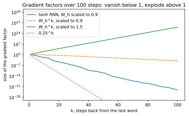
What the 100-step products show
- The tanh RNN's factor falls to 8.3 × 10⁻²⁴ after 100 steps: the first word's term in the gradient is gone.
- Wh scaled to 0.9 falls more slowly, to 9.5 × 10⁻⁵: the tanh derivatives, each at most 1, are what pull the real RNN down so much further.
- Wh scaled to 1.5 grows to 1.5 × 10¹⁸: that is the exploding gradient. Updates that large throw the weights far away and the loss turns into
nan. - 0.25k is the sigmoid's best case and falls fastest of all.
Exploding gradients and gradient clipping
Exploding gradients have a simple fix (Pascanu et al., 2013): before each update, if the gradient's size (its L2 norm) is above a threshold c, scale it down to size c. The direction stays the same; only the step gets shorter.
import numpy as np

def clip_by_norm(g, max_norm):
    norm = np.linalg.norm(g)
    return g * (max_norm / norm) if norm > max_norm else g

g = np.array([30.0, 40.0])                 # an exploding gradient, size 50
print("before:", g, "size", np.linalg.norm(g))
clipped = clip_by_norm(g, 5.0)
print("after: ", clipped, "size", np.linalg.norm(clipped))
small = np.array([0.3, 0.4])
print("a small gradient is left alone:", clip_by_norm(small, 5.0))before: [30. 40.] size 50.0 after: [3. 4.] size 5.0 a small gradient is left alone: [0.3 0.4]
- The gradient [30, 40] has size 50; clipped to 5 it becomes [3, 4], the same direction.
- A gradient already below the threshold passes through unchanged.
In Keras the optimizer clips for you:
import keras

optimizer = keras.optimizers.Adam(learning_rate=1e-3, clipnorm=1.0)   # clip each gradient to size 1
model.compile(loss="binary_crossentropy", optimizer=optimizer, metrics=["accuracy"])
Vanishing vs exploding gradients
| Vanishing | Exploding | |
|---|---|---|
| Step factor | size below 1 | size above 1 |
| What you see | early words never matter; loss stalls | loss jumps or becomes nan |
| Fix | gated cells: LSTM, GRU | gradient clipping, a smaller learning rate |
| Easy to spot? | no, training runs quietly | yes, the numbers blow up |
Where you use these ideas
- Choosing an LSTM or GRU over a plain RNN for any text longer than a short phrase.
- Setting
clipnormwhen training recurrent models, as a guard against spikes. - Reading a training log: a loss of
nanafter a few batches points to exploding gradients.
Related
- Previous: Backpropagation through time (BPTT)
- Next: LSTM (long short-term memory)
- See also: Vanishing gradient problem
- Change
W_big = 1.5 * Rto1.0 * Rand see the third curve flatten. - Run the 100-step tanh RNN with
W_biginstead ofW_smalland check whether the tanh derivatives keep the product from exploding. - Call
clip_by_norm(g, 100.0)and confirm that a gradient of size 50 is not changed.
Slow is fine. Stopping is the only problem.