
Spam classifier with BoW and TF-IDF
A spam classifier is a text classification model that reads a message and labels it spam or ham (an ordinary message). This one turns 5,572 SMS messages into bag of words and TF-IDF vectors and trains a multinomial naive Bayes model on them.
Last updated: 07 Oct, 2026 · NLTK 3.10 · scikit-learn 1.9
The Bag of words (BoW) and TF-IDF lessons turned three short sentences into vectors by hand. This project runs the same encodings on a real dataset, feeds the vectors to a model and measures how well it separates spam from ham.
Planning the spam classification project
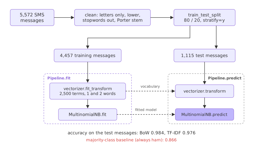
The plan in the video has three stages. Text preprocessing comes first: tokenize the messages, remove stopwords and reduce each word with stemming or lemmatization. Then the text becomes vectors with bag of words, TF-IDF or Word2Vec. Last, a machine learning algorithm trains on the vectors and its accuracy is measured.
Two steps make the measurement honest. The data is split into training and test messages before any vectorizer learns a vocabulary, and the accuracy is compared with a model that always predicts the most common class. This lesson builds the BoW and TF-IDF versions; the Word2Vec version is the next lesson.
Loading the SMS Spam Collection
The SMS Spam Collection comes from the UCI Machine Learning Repository. It is one tab-separated text file: each line holds a label, ham or spam, a tab and the message. read_csv with sep="\t" and two column names reads it straight from the materials repo on GitHub, so nothing needs downloading by hand.
import pandas as pd

URL = ("https://raw.githubusercontent.com/krishnaik06/The-Grand-Complete-Data-Science-Materials/main/"
       "Complete%20NLP%20For%20ML%20%26%20Deep%20Learning/Practicals/SpamClassifier-master/smsspamcollection/SMSSpamCollection")
messages = pd.read_csv(URL, sep="\t", names=["label", "message"])

print(messages.shape)
print(messages["label"].value_counts().to_dict())
print(messages.loc[2, "message"])
print("share of ham:", round((messages["label"] == "ham").mean(), 4))(5572, 2)
{'ham': 4825, 'spam': 747}
Free entry in 2 a wkly comp to win FA Cup final tkts 21st May 2005. Text FA to 87121 to receive entry question(std txt rate)T&C's apply 08452810075over18's
share of ham: 0.8659- 5,572 messages in two columns,
labelandmessage. - 4,825 are ham and 747 are spam, so 86.59% of all messages are ham. A model that always answers ham is already right 86.59% of the time, and every accuracy in this project has to be read against that number.
- Message 2 is a typical spam text: a prize, a short code to text and a price per message.
Cleaning the messages with stemming
Each message goes through the steps of the Stopwords and Stemming lessons. A regular expression replaces every character that is not a letter, [^a-zA-Z], with a space. The text is lower-cased and split into words, the NLTK English stopwords are dropped, and the Porter stemmer cuts each word to its stem. The stopword list is turned into a set once, because checking a word against a set is fast and the check runs for every word of every message.
The stopword list is an NLTK resource. Download it once:
import nltk
nltk.download("stopwords")import re
from nltk.corpus import stopwords
from nltk.stem import PorterStemmer
ps = PorterStemmer()
stop = set(stopwords.words("english")) # a set, built once, for fast lookups
def clean(text):
words = re.sub("[^a-zA-Z]", " ", text).lower().split() # letters only, lower case
return " ".join(ps.stem(w) for w in words if w not in stop)
corpus = messages["message"].apply(clean)
print(corpus[0])go jurong point crazi avail bugi n great world la e buffet cine got amor wat
The first message, "Go until jurong point, crazy.. Available only in bugis n great world la e buffet... Cine there got amore wat...", keeps 16 stems. "until", "only", "in" and "there" are stopwords, and "crazy" and "available" become the stems crazi and avail.
Coding the labels as 0 and 1
A model needs numbers for the labels. Here spam is 1 and ham is 0, so row 1 of every report below is the spam class, the one the filter exists for. The project notebooks build the label with pd.get_dummies(messages['label']).iloc[:, 0], which picks the ham column, so in their reports 1 means ham.
y = (messages["label"] == "spam").astype(int) # spam = 1, ham = 0Choosing the bag of words settings
CountVectorizer builds the bag of words. max_features=2500 keeps the 2,500 terms that occur most often across the messages and drops the rest, so every message becomes a vector of length 2,500. With binary=True a word that appears twice in a message still counts 1; without it the cell holds the count. ngram_range adds groups of neighbouring words as extra terms (see N-grams).
The live session uses binary=True and single words. The project notebook for this lesson (27.2 in the materials repo) keeps the counts and sets ngram_range=(1, 2), so pairs such as free entri and claim call become features of their own. The code here follows notebook 27.2.
Splitting before fitting the vectorizer
Data leakage is information from the test data reaching the model during training. A vectorizer fitted on all 5,572 messages has chosen its 2,500 terms, and for TF-IDF its idf weights, partly from the test messages. The test score then measures a model that has already seen the test vocabulary. The live session fits the vectorizer on every message to keep the demo short and recommends splitting first and fitting on the training part only; notebook 27.2 does that, and so does the code here.
train_test_split keeps 20% of the messages for testing (see Train and test split). stratify=y keeps the spam share the same, about 13.4%, in both parts, and random_state=42 makes the split the same on every run.
from sklearn.model_selection import train_test_split

X_train, X_test, y_train, y_test = train_test_split(
    corpus, y, test_size=0.20, random_state=42, stratify=y)   # same spam share in both parts
Putting the vectorizer and the model in a Pipeline
A Pipeline chains the steps into one estimator. fit() fits the vectorizer on X_train and the model on the vectorizer's output; predict() only transforms new messages with the fitted vocabulary. The leak cannot happen by accident. The model is MultinomialNB, the Naive Bayes variant that models how often each term appears in each class, which is what count vectors hold. scikit-learn's MultinomialNB takes the sparse matrix the vectorizer returns, so .toarray() is not needed.
from sklearn.pipeline import Pipeline
from sklearn.feature_extraction.text import CountVectorizer
from sklearn.naive_bayes import MultinomialNB

bow_model = Pipeline([
    ("bow", CountVectorizer(max_features=2500, ngram_range=(1, 2))),
    ("nb", MultinomialNB()),
])
bow_model.fit(X_train, y_train)       # the vocabulary comes from the training messages only
y_pred = bow_model.predict(X_test)    # the test messages are only transformed
Measuring against a majority-class baseline
DummyClassifier(strategy="most_frequent") always predicts the class it saw most in training, here ham. Its accuracy is the floor a real model must beat. classification_report takes the true labels first and the predictions second.
from sklearn.dummy import DummyClassifier
from sklearn.metrics import accuracy_score, classification_report

baseline = DummyClassifier(strategy="most_frequent").fit(X_train, y_train)
print(accuracy_score(y_test, baseline.predict(X_test)))     # always predicts ham
print(classification_report(y_test, y_pred, target_names=["ham", "spam"]))   # true labels first
Training the BoW and TF-IDF spam models
The full run trains both encodings with the same split, the same 2,500 terms of one and two words, and the same model, so the only difference is what each cell of the vector holds.
from sklearn.model_selection import train_test_split
from sklearn.pipeline import Pipeline
from sklearn.feature_extraction.text import CountVectorizer, TfidfVectorizer
from sklearn.naive_bayes import MultinomialNB
from sklearn.dummy import DummyClassifier
from sklearn.metrics import accuracy_score, classification_report, confusion_matrix

y = (messages["label"] == "spam").astype(int)     # spam = 1, ham = 0
X_train, X_test, y_train, y_test = train_test_split(
    corpus, y, test_size=0.20, random_state=42, stratify=y)
print("train:", len(X_train), "test:", len(X_test), "spam in test:", y_test.sum())

baseline = DummyClassifier(strategy="most_frequent").fit(X_train, y_train)
print("majority-class baseline:", round(accuracy_score(y_test, baseline.predict(X_test)), 4))

models = {}
for name, vectorizer in [("BoW", CountVectorizer(max_features=2500, ngram_range=(1, 2))),
                         ("TF-IDF", TfidfVectorizer(max_features=2500, ngram_range=(1, 2)))]:
    models[name] = Pipeline([("vec", vectorizer), ("nb", MultinomialNB())]).fit(X_train, y_train)
    y_pred = models[name].predict(X_test)
    print(f"\n{name} + MultinomialNB accuracy:", round(accuracy_score(y_test, y_pred), 4))
    print(confusion_matrix(y_test, y_pred))
print(classification_report(y_test, y_pred, target_names=["ham", "spam"], digits=3))train: 4457 test: 1115 spam in test: 149
majority-class baseline: 0.8664
BoW + MultinomialNB accuracy: 0.9839
[[962 4]
[ 14 135]]
precision recall f1-score support
ham 0.986 0.996 0.991 966
spam 0.971 0.906 0.938 149
accuracy 0.984 1115
macro avg 0.978 0.951 0.964 1115
weighted avg 0.984 0.984 0.984 1115
TF-IDF + MultinomialNB accuracy: 0.9758
[[965 1]
[ 26 123]]
precision recall f1-score support
ham 0.974 0.999 0.986 966
spam 0.992 0.826 0.901 149
accuracy 0.976 1115
macro avg 0.983 0.912 0.944 1115
weighted avg 0.976 0.976 0.975 1115What the two reports show
- The baseline scores 0.8664: the test part holds 966 ham and 149 spam messages, and 966 / 1,115 = 0.8664.
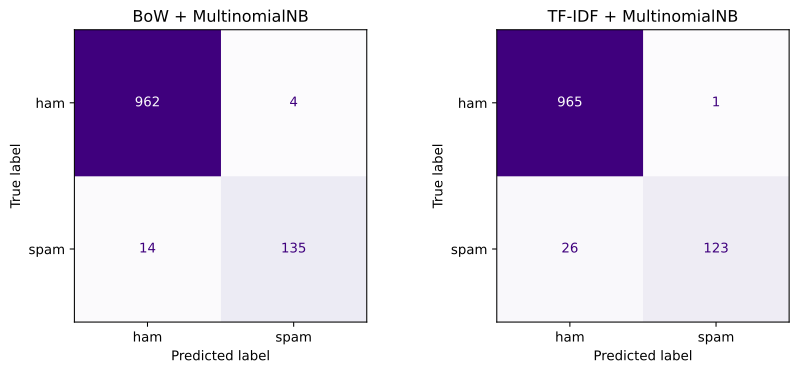
- BoW + MultinomialNB reaches 0.9839, 11.75 points above the baseline. Its confusion matrix shows 135 of the 149 spam messages caught (recall 0.906) and 4 ham messages flagged as spam (spam precision 0.971).
- TF-IDF + MultinomialNB reaches 0.9758. It flags only 1 ham message, so its spam precision is 0.992, but it misses 26 spam messages, so its spam recall drops to 0.826.
- On this data, BoW is the better input for MultinomialNB. The two models differ in the spam they miss, 14 against 26, far more than in the ham they flag.
- The ham rows look perfect in both (recall 0.996 and 0.999) because ham is the easy majority class. The spam row is where the two models differ.
import matplotlib.pyplot as plt
from sklearn.metrics import ConfusionMatrixDisplay, confusion_matrix

fig, axes = plt.subplots(1, 2, figsize=(9, 4))
for ax, (name, model) in zip(axes, models.items()):
    ConfusionMatrixDisplay.from_estimator(model, X_test, y_test, display_labels=["ham", "spam"],
                                          ax=ax, colorbar=False, cmap="Purples")
    ax.set_title(name + " + MultinomialNB")
    print(name, "[tn, fp, fn, tp]:", confusion_matrix(y_test, model.predict(X_test)).ravel().tolist())
plt.tight_layout()
plt.show()BoW [tn, fp, fn, tp]: [962, 4, 14, 135] TF-IDF [tn, fp, fn, tp]: [965, 1, 26, 123]
Reading precision and recall the right way round
classification_report(y_true, y_pred) groups the messages by their true class. Spam precision is the share of messages predicted spam that are spam; spam recall is the share of true spam messages the model caught; support is the number of true messages in each class (see Precision, recall and F-beta). With the arguments swapped, scikit-learn treats the predictions as the truth: precision and recall trade places and support counts the predictions.
y_pred = models["BoW"].predict(X_test)
print("classification_report(y_test, y_pred):")
print(classification_report(y_test, y_pred, target_names=["ham", "spam"], digits=3))
print("classification_report(y_pred, y_test), arguments swapped:")
print(classification_report(y_pred, y_test, target_names=["ham", "spam"], digits=3))classification_report(y_test, y_pred):
precision recall f1-score support
ham 0.986 0.996 0.991 966
spam 0.971 0.906 0.938 149
accuracy 0.984 1115
macro avg 0.978 0.951 0.964 1115
weighted avg 0.984 0.984 0.984 1115
classification_report(y_pred, y_test), arguments swapped:
precision recall f1-score support
ham 0.996 0.986 0.991 976
spam 0.906 0.971 0.938 139
accuracy 0.984 1115
macro avg 0.951 0.978 0.964 1115
weighted avg 0.985 0.984 0.984 1115- The correct report gives spam precision 0.971, recall 0.906 and support 149, the number of spam messages in the test part.
- The swapped report gives spam precision 0.906 and recall 0.971, and its support of 139 is the number of messages the model predicted as spam (135 + 4).
- The accuracy, 0.984, is the same in both, which is why the swap goes unnoticed. For a spam filter the difference matters: 0.906 recall means about 1 spam in 11 reaches the inbox.
BoW vs TF-IDF for spam
| BoW (CountVectorizer) | TF-IDF (TfidfVectorizer) | |
|---|---|---|
| Cell value | how often the term appears in the message | count × smoothed idf, each row scaled to length 1 |
| Terms kept here | 2,500 most frequent unigrams and bigrams | the same 2,500 terms |
| Accuracy here (MultinomialNB) | 0.9839 | 0.9758 |
| Spam caught (recall) | 135 of 149 (0.906) | 123 of 149 (0.826) |
| Ham flagged as spam | 4 | 1 |
| Helps most when | frequent words carry the signal | common words drown out rarer, telling ones |
Where you use a spam classifier
- SMS and email filtering, where a message predicted spam goes to a separate folder instead of the inbox.
- Comment and review moderation, to hold back promotional or scam posts for a human to check.
- A first text-classification baseline: BoW or TF-IDF with naive Bayes trains in under a second and sets the score that a heavier model has to beat.
Pipeline does for you. A vectorizer fitted before the split chooses its terms and idf weights partly from the test messages. And read every accuracy next to the 0.866 baseline: with 13% spam, the spam recall says more about the filter than the overall accuracy.Related
- Previous: Average Word2Vec
- Next: Spam classifier with Average Word2Vec
- See also: Naive Bayes, Confusion matrix
- Reference: Pipeline in the scikit-learn user guide
- Add
binary=Trueto the CountVectorizer, as in the live session, and compare the spam recall with the count version. - Change
ngram_range=(1, 2)to(1, 1)in both vectorizers and see whether the bigrams were helping. - Replace
MultinomialNB()withLogisticRegression(max_iter=1000)fromsklearn.linear_modeland read how the spam precision and recall move.
You understood something today that you didn't yesterday.