
Linear and softmax output layer
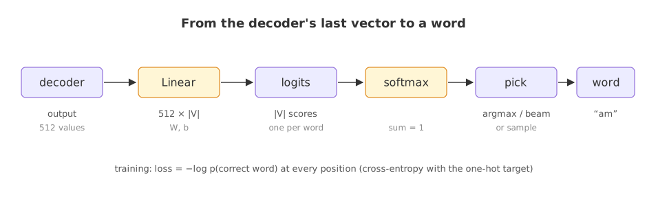
The linear and softmax output layer is the last step of the transformer decoder that turns each output vector into a probability for every word in the vocabulary, so the model can pick the next word.
Last updated: 07 Oct, 2026 · NumPy
After Cross-attention (encoder-decoder attention) and the last feed-forward network, the decoder stack still outputs vectors of 512 numbers. A translation needs words. This layer is the bridge.
Projecting the decoder vector to logits
The linear layer is a simple fully connected neural network that projects the vector produced by the stack of decoders into a much larger vector called the logits vector. If the model knows 10,000 unique words, its vocabulary, the logits vector is 10,000 cells wide, and each cell is the score of one unique word.
In the paper dmodel = 512, and the vocabularies are subword tokens rather than words: about 37,000 byte-pair tokens shared between English and German, and 32,000 word-pieces for English-French. The paper also ties this layer's weight matrix to the embedding matrices, so the same table that turns a token into a vector turns a vector back into token scores.
Turning logits into probabilities with softmax
The softmax layer turns those scores into probabilities that all add up to 1.0, the usual multi-class classification step (Softmax). The cell with the highest probability is chosen, and the word associated with it is produced as the output for that time step. For the loss and for beam search the model works with the logarithm of these probabilities, the log-probabilities, given directly by log-softmax.
Training the output layer with cross-entropy
The recap of training uses a six-word output vocabulary: a = 0, am = 1, I = 2, thanks = 3, student = 4, <eos> = 5. The one-hot encoding of “am” is [0, 1, 0, 0, 0, 0]. For the French word “merci” the correct output is “thanks”, [0, 0, 0, 1, 0, 0], while an untrained model might output [0.2, 0.2, 0.1, 0.2, 0.2, 0.1]. The loss function compares the two, and backpropagation adjusts the weights to reduce it.
The loss is cross-entropy with the one-hot target, which reduces to −log of the probability given to the correct word (Categorical cross-entropy). For a whole sentence it is computed at every position. For “je suis étudiant” the target is “I am a student <eos>”, and after training the outputs per position look like this (rounded, illustrative values):
| Position | a | am | I | thanks | student | <eos> |
|---|---|---|---|---|---|---|
| 1 | 0.01 | 0.02 | 0.93 | 0.01 | 0.03 | 0.01 |
| 2 | 0.01 | 0.80 | 0.10 | 0.05 | 0.01 | 0.03 |
| 3 | 0.99 | 0.001 | 0.001 | 0.001 | 0.002 | 0.001 |
| 4 | 0.001 | 0.002 | 0.001 | 0.02 | 0.94 | 0.01 |
| 5 | 0.01 | 0.01 | 0.001 | 0.001 | 0.001 | 0.98 |
The paper trains with label smoothing of 0.1: the one-hot target is mixed with a uniform distribution, so 0.9 of the weight stays on the correct word and the remaining 0.1 is spread evenly over the whole vocabulary, which makes the model less over-confident.
Choosing the word: greedy, beam search and sampling
- Greedy decoding takes the highest-probability word at each step, the rule described in the clip.
- Beam search keeps the k best partial sentences at each step and picks the best complete one. The paper uses a beam of 4 with a length penalty α = 0.6.
- Sampling draws the word at random from the probabilities. A temperature T divides the logits first (T < 1 sharpens, T > 1 flattens), and top-k or top-p keeps only the most likely words before drawing. Chat models mostly sample.
Scoring the board's outputs with cross-entropy
import numpy as np

vocab = ["a", "am", "I", "thanks", "student", "<eos>"]
target = ["I", "am", "a", "student", "<eos>"]

untrained = np.array([0.2, 0.2, 0.1, 0.2, 0.2, 0.1])          # output for "merci" before training
print("untrained loss for 'thanks':", round(-np.log(untrained[vocab.index("thanks")]), 4))

trained = np.array([[0.01, 0.02, 0.93, 0.01, 0.03, 0.01],
                    [0.01, 0.80, 0.10, 0.05, 0.01, 0.03],
                    [0.99, 0.001, 0.001, 0.001, 0.002, 0.001],
                    [0.001, 0.002, 0.001, 0.02, 0.94, 0.01],
                    [0.01, 0.01, 0.001, 0.001, 0.001, 0.98]])
picked = [vocab[i] for i in trained.argmax(axis=1)]
loss = [-np.log(row[vocab.index(w)]) for row, w in zip(trained, target)]
print("argmax per position:", picked)
print("loss per position:", np.round(loss, 4))
print("mean loss:", round(float(np.mean(loss)), 4))untrained loss for 'thanks': 1.6094 argmax per position: ['I', 'am', 'a', 'student', '<eos>'] loss per position: [0.0726 0.2231 0.0101 0.0619 0.0202] mean loss: 0.0776
- The untrained loss for “thanks” is 1.6094, −ln 0.2: the model gave the right word only 0.2.
- argmax reads back “I am a student <eos>” from the trained table, position by position.
- The losses are 0.0726, 0.2231, 0.0101, 0.0619 and 0.0202; position 2 is the highest because “am” got 0.80. The mean is 0.0776, about one twentieth of the untrained loss.
Decoding from one logits vector
A random decoder vector and a random linear layer over the same six words. Nothing is trained, so the chosen word means nothing; the point is what each decoding rule does with the same logits.
import numpy as np

vocab = ["a", "am", "I", "thanks", "student", "<eos>"]
rng = np.random.default_rng(42)
d_model = 4

h = rng.normal(0, 1, d_model)                     # one decoder output vector
W = rng.normal(0, 1, (d_model, len(vocab)))        # the linear layer: d_model -> vocabulary
b = np.zeros(len(vocab))

def softmax(z, T=1.0):
    e = np.exp((z - z.max()) / T)
    return e / e.sum()

logits = h @ W + b
p = softmax(logits)
print("logits:       ", np.round(logits, 3))
print("probabilities:", np.round(p, 3), " sum", round(p.sum(), 6))
print("log-probs:    ", np.round(np.log(p), 3))
print("greedy pick:  ", vocab[p.argmax()])
for T in (0.5, 2.0):
    print(f"temperature {T}:", np.round(softmax(logits, T), 3))

top3 = np.argsort(p)[::-1][:3]                     # top-k sampling with k = 3
p3 = p[top3] / p[top3].sum()
draws = rng.choice(top3, size=8, p=p3)
print("top-3 words:", [vocab[i] for i in top3], " renormalised", np.round(p3, 3))
print("8 samples: ", [vocab[i] for i in draws])logits: [-0.082 -2.071 0.227 -1.637 -0.129 0.466] probabilities: [0.185 0.025 0.252 0.039 0.177 0.321] sum 1.0 log-probs: [-1.686 -3.674 -1.377 -3.241 -1.733 -1.137] greedy pick: <eos> temperature 0.5: [0.146 0.003 0.272 0.007 0.133 0.439] temperature 2.0: [0.189 0.07 0.221 0.087 0.185 0.249] top-3 words: ['<eos>', 'I', 'a'] renormalised [0.423 0.333 0.244] 8 samples: ['<eos>', 'I', 'I', 'a', '<eos>', '<eos>', 'I', '<eos>']
- The probabilities sum to 1, and their logs are the log-probabilities, all negative.
- Greedy picks <eos>, the largest logit, 0.466 (probability 0.321).
- Temperature 0.5 raises <eos> to 0.439; temperature 2.0 flattens it to 0.249.
- Top-3 sampling keeps <eos>, I and a, renormalises them to 0.423, 0.333 and 0.244, and draws a different word on different draws.
Greedy vs beam search on a two-step choice
# two decoding steps; each entry is P(next word | words so far)
step1 = {"I": 0.5, "Thanks": 0.4, "a": 0.1}
step2 = {"I": {"am": 0.4, "is": 0.35, "a": 0.25},
         "Thanks": {"<eos>": 0.9, "a": 0.1},
         "a": {"student": 1.0}}

w1 = max(step1, key=step1.get)                     # greedy: best first word
w2 = max(step2[w1], key=step2[w1].get)             # then best second word
print("greedy:", w1, w2, " probability", round(step1[w1] * step2[w1][w2], 3))

beam = sorted(step1, key=step1.get, reverse=True)[:2]          # beam of width 2
cands = [(a, b, step1[a] * pb) for a in beam for b, pb in step2[a].items()]
best = max(cands, key=lambda c: c[2])
print("beam 2:", best[0], best[1], " probability", round(best[2], 3))greedy: I am probability 0.2 beam 2: Thanks <eos> probability 0.36
- Greedy takes “I” (0.5) and then “am” (0.4): 0.5 × 0.4 = 0.2.
- A beam of 2 also keeps “Thanks” (0.4), whose next word <eos> has 0.9: 0.4 × 0.9 = 0.36, the more likely sentence. Greedy cannot recover from its first choice; a beam can.
Greedy vs beam search vs sampling
| Greedy | Beam search | Sampling (temperature, top-k, top-p) | |
|---|---|---|---|
| Picks | the top word each step | the best of k running sentences | a random word by probability |
| Same input, same output | yes | yes | no (unless seeded) |
| Cost | 1 pass per token | about k passes per token | 1 pass per token |
| Good for | short, factual outputs | translation, summarization | chat, creative text |
Where you use the linear and softmax output layer
- Every generative transformer: GPT, T5 and translation models end in this projection to the vocabulary.
- Classification heads: the same linear + softmax with one cell per class instead of per word.
- Language-model scoring: the log-probabilities of a sentence's tokens give its likelihood.
np.exp(logits) directly overflows for large logits. Subtract the maximum logit first, as the softmax above does; it does not change the probabilities. And for greedy decoding there is no need for softmax at all: argmax of the logits is the same word.Related
- Previous: Cross-attention (encoder-decoder attention)
- Next: Subword tokenization (BPE and WordPiece)
- See also: Softmax
- Change the untrained output so that “thanks” gets 0.5 (and another word 0.0) and recompute its loss.
- Set the temperature to 0.1 and to 10 in the decoding example and describe both extremes.
- In the beam example, change
"<eos>": 0.9to0.45and see whether greedy and beam agree.
Slow is fine. Stopping is the only problem.