
Sentiment analysis of Kindle reviews
Sentiment analysis is a text classification task that labels a text by the opinion it expresses, here positive or negative. This project predicts it for 12,000 Amazon Kindle book reviews and compares bag of words, TF-IDF and Average Word2Vec features.
Last updated: 07 Oct, 2026 · NLTK 3.10 · scikit-learn 1.9
The Spam classifier with Average Word2Vec lesson ended a two-part spam project. This project asks a different question of longer texts: does the reviewer like the book? The steps are the same ones, preprocessing, a split, vectors and a model, and two of them need more care here: the order of the cleaning steps and the choice of model for each kind of vector.
Loading the Kindle review data
The data is a 12,000-review sample of the Amazon Kindle Store reviews collected between May 1996 and July 2014, a 5-core dataset (every reviewer and every book has at least 5 reviews) of 982,619 reviews in full. Each row has the review text, the star rating from 1 to 5 and columns such as the product id and the review time. The project keeps reviewText and rating.
A rating of 3 or more counts as positive (1) and 1 or 2 as negative (0), the mapping of the project notebook. Rating 3 is the neutral middle, so a 3-star review counts as positive here; one Try it item drops the 3s instead.
import pandas as pd

URL = ("https://raw.githubusercontent.com/krishnaik06/The-Grand-Complete-Data-Science-Materials/main/"
       "Complete%20NLP%20For%20ML%20%26%20Deep%20Learning/Kindle%20Reviews/all_kindle_review.csv")
data = pd.read_csv(URL)
df = data[["reviewText", "rating"]].copy()
df["label"] = (df["rating"] >= 3).astype(int)     # 1 = positive (3, 4, 5), 0 = negative (1, 2)

print(df.shape, "| missing:", df[["reviewText", "rating"]].isnull().sum().to_dict())
print("ratings:", df["rating"].value_counts().sort_index().to_dict())
print("labels:", df["label"].value_counts().to_dict(), "| share positive:", round(df["label"].mean(), 4))(12000, 3) | missing: {'reviewText': 0, 'rating': 0}
ratings: {1: 2000, 2: 2000, 3: 2000, 4: 3000, 5: 3000}
labels: {1: 8000, 0: 4000} | share positive: 0.6667- 12,000 reviews with no missing text or rating.
- The ratings are balanced by design: 2,000 each for 1, 2 and 3 stars and 3,000 each for 4 and 5.
- 8,000 positive and 4,000 negative after the mapping, so two thirds of the reviews are positive. Always answering "positive" scores 0.6667.
Cleaning reviews in the right order
Reviews are messier than SMS messages. A few contain links ("located at http://www.amazon.com/gp/daily"), and many contain HTML entities: " is how the page stored a double quote. The steps are those of the Text cleaning and normalisation lesson, and their order matters. A URL pattern looks for :// and an HTML tag for < and >, so both must run before the step that deletes special characters. The order here is:
- lower-case the text;
- remove URLs;
- remove HTML tags and decode entities such as
"; - replace every character other than a letter, digit, space or hyphen with a space;
- drop the stopwords and lemmatize the rest.
These reviews need stopwords and WordNet:
import nltk
nltk.download("stopwords")
nltk.download("wordnet")
nltk.download("omw-1.4")import re
import html
from nltk.corpus import stopwords
from nltk.stem import WordNetLemmatizer
stop = set(stopwords.words("english"))
lemmatizer = WordNetLemmatizer()
def clean(text):
text = text.lower()
text = re.sub(r"(https?|ftp)://\S+|www\.\S+", " ", text) # 2. URLs, while ':' and '/' exist
text = html.unescape(re.sub(r"<[^>]+>", " ", text)) # 3. HTML tags, then " becomes "
text = re.sub(r"[^a-z0-9\s-]", " ", text) # 4. special characters
return " ".join(lemmatizer.lemmatize(w) for w in text.split() if w not in stop)The project notebook removes tags and entities with BeautifulSoup, which does both jobs of step 3 in one call; html.unescape and a tag regex do the same without the extra package:
from bs4 import BeautifulSoup                      # pip install beautifulsoup4 lxml
text = BeautifulSoup(text, "lxml").get_text()      # removes tags and decodes " in one call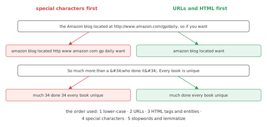
Comparing the two cleaning orders
The run below cleans two fragments of real reviews both ways, then cleans all 12,000 reviews in the right order. The wrong-order function uses the same regular expressions; only the order differs.
def clean_special_first(text): # the same steps, special characters first
text = re.sub(r"[^a-z0-9\s-]", " ", text.lower())
text = re.sub(r"(https?|ftp)://\S+|www\.\S+", " ", text) # finds nothing now
text = html.unescape(re.sub(r"<[^>]+>", " ", text))
return " ".join(lemmatizer.lemmatize(w) for w in text.split() if w not in stop)
has_url = df["reviewText"].str.contains("http")
has_entity = df["reviewText"].str.contains(r"&#?\w+;")
print("reviews with a URL:", has_url.sum(), "| with an HTML entity such as ":", has_entity.sum())
samples = ["the Amazon blog located at http://www.amazon.com/gp/daily, so if you want",
"So much more than a "who done it". Every book is unique"]
for s in samples:
print("\n", s)
print(" special characters first:", clean_special_first(s))
print(" URLs and HTML first: ", clean(s))
df["clean"] = df["reviewText"].apply(clean)
print("\nreview 1 cleaned:", df.loc[1, "clean"])reviews with a URL: 7 | with an HTML entity such as ": 587 the Amazon blog located at http://www.amazon.com/gp/daily, so if you want special characters first: amazon blog located http www amazon com gp daily want URLs and HTML first: amazon blog located want So much more than a "who done it". Every book is unique special characters first: much 34 done 34 every book unique URLs and HTML first: much done every book unique review 1 cleaned: great short read want put read one sitting sex scene great two male one female character bit surprising - never thought could learned something new really enjoyed reading book great way get hot bothered take advantage significant
- 7 reviews contain a URL and 587 an HTML entity, enough to put junk tokens into the vocabulary.
- Special characters first turns the link into the six tokens
http www amazon com gp dailyand the entity into the token34, because the URL pattern has nothing left to match. - URLs and HTML first remove the link and decode
"into a quote mark, which step 4 then deletes, so no number is left behind. - Review 1 keeps its opinion words, "great short read", "enjoyed", after the stopwords are dropped.
Choosing a model for each feature set
Each kind of vector suits a different model. MultinomialNB models word counts, so it fits bag of words. TF-IDF cells are small fractions, scaled so that each row has length 1, and Logistic regression learns a weight per word from them. GaussianNB assumes each feature follows a bell curve around a class mean; a word count is 0 in almost every review, far from a bell curve. The project notebook trains GaussianNB on both BoW and TF-IDF; the comparison below includes it next to the other models and the majority-class baseline.
The last row uses Average Word2Vec features: the AvgWord2Vec transformer from the Spam classifier with Average Word2Vec lesson, trained for 20 epochs on the training reviews, with logistic regression on top. GaussianNB needs a dense matrix, so FunctionTransformer converts the counts with .toarray(); that matrix takes close to 1 GB of memory.
import numpy as np
import matplotlib.pyplot as plt
from sklearn.model_selection import train_test_split
from sklearn.pipeline import Pipeline
from sklearn.preprocessing import FunctionTransformer
from sklearn.feature_extraction.text import CountVectorizer, TfidfVectorizer
from sklearn.naive_bayes import GaussianNB, MultinomialNB
from sklearn.linear_model import LogisticRegression
from sklearn.metrics import accuracy_score, confusion_matrix

X_train, X_test, y_train, y_test = train_test_split(
    df["clean"], df["label"], test_size=0.20, random_state=42, stratify=df["label"])
baseline = y_test.value_counts(normalize=True).max()
dense = FunctionTransformer(lambda X: X.toarray().astype(np.float32), accept_sparse=True)

models = {
    "BoW + GaussianNB": Pipeline([("bow", CountVectorizer()), ("dense", dense), ("nb", GaussianNB())]),
    "BoW + MultinomialNB": Pipeline([("bow", CountVectorizer()), ("nb", MultinomialNB())]),
    "TF-IDF + MultinomialNB": Pipeline([("tfidf", TfidfVectorizer()), ("nb", MultinomialNB())]),
    "TF-IDF + logistic regression": Pipeline([("tfidf", TfidfVectorizer()),
                                              ("lr", LogisticRegression(max_iter=1000))]),
}
scores = {}
for name, model in models.items():
    y_pred = model.fit(X_train, y_train).predict(X_test)
    scores[name] = accuracy_score(y_test, y_pred)
    if name.startswith("TF-IDF"):
        print(name, "confusion matrix:", confusion_matrix(y_test, y_pred).tolist())

tok_train, tok_test = [t.split() for t in X_train], [t.split() for t in X_test]
w2v = Pipeline([("avg_w2v", AvgWord2Vec(epochs=20)), ("lr", LogisticRegression(max_iter=2000))])
scores["AvgWord2Vec + logistic regression"] = accuracy_score(y_test, w2v.fit(tok_train, y_train).predict(tok_test))

print("\ntest reviews:", len(X_test), "| majority-class baseline:", round(baseline, 4))
for name, s in scores.items():
    print(f"{name:34s} {s:.4f}")

plt.figure(figsize=(8, 3.8))
plt.barh(list(scores), list(scores.values()), color="#9370DB")
plt.axvline(baseline, color="#d64541", linestyle="--", label=f"majority class {baseline:.3f}")
plt.xlim(0.4, 0.9)
plt.xlabel("test accuracy")
plt.title("Kindle review sentiment, 2,400 test reviews")
plt.legend(loc="upper right")
plt.gca().invert_yaxis()
plt.tight_layout()
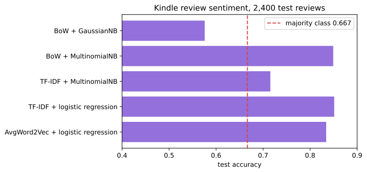
plt.show()TF-IDF + MultinomialNB confusion matrix: [[123, 677], [6, 1594]] TF-IDF + logistic regression confusion matrix: [[532, 268], [89, 1511]] test reviews: 2400 | majority-class baseline: 0.6667 BoW + GaussianNB 0.5758 BoW + MultinomialNB 0.8492 TF-IDF + MultinomialNB 0.7154 TF-IDF + logistic regression 0.8512 AvgWord2Vec + logistic regression 0.8342
What the comparison shows
- BoW + GaussianNB scores 0.5758, below the 0.6667 baseline. The model is the problem, not the vectors: the same counts give 0.8492 with MultinomialNB.
- TF-IDF + logistic regression is the best, 0.8512, with BoW + MultinomialNB close behind at 0.8492.
- TF-IDF + MultinomialNB scores 0.7154. Its confusion matrix shows the problem: it calls 677 of the 800 negative reviews positive and leans to the majority class. Logistic regression on the same features finds 532 of the 800 negatives.
- AvgWord2Vec + logistic regression reaches 0.8342. An average over every word of a review gives its few opinion words little weight, and it trails the word-level features.
GaussianNB vs MultinomialNB vs logistic regression
| GaussianNB | MultinomialNB | Logistic regression | |
|---|---|---|---|
| Assumes | each feature is normal within a class | features are counts of words | a weighted sum of features separates the classes |
| Fits | continuous measurements | BoW counts | TF-IDF, BoW, dense vectors |
| Input here | dense array, about 1 GB | sparse counts | sparse or dense |
| Accuracy here | 0.5758 (BoW) | 0.8492 (BoW), 0.7154 (TF-IDF) | 0.8512 (TF-IDF), 0.8342 (AvgWord2Vec) |
Where you use sentiment analysis
- Product and book reviews, to track how opinion about an item changes and to surface the negative reviews first.
- Support tickets and survey answers, to route angry messages to a person sooner.
- Social media monitoring, to measure how people talk about a brand or an event over time.
34 in the vocabulary.Related
- Previous: Spam classifier with Average Word2Vec
- Next: Recurrent neural network (RNN)
- See also: TF-IDF, Naive Bayes
- Reference: Naive Bayes in the scikit-learn user guide
- Drop the neutral reviews with
df = df[df["rating"] != 3]before the split and see how the baseline and the best accuracy change. - Give the TF-IDF vectorizer
ngram_range=(1, 2)so that "not good" becomes a feature, and compare the logistic regression score. - Add
class_weight="balanced"toLogisticRegressionand read the new confusion matrix for the negative reviews.
This is what real progress feels like.