
LSTM text classification (fake news)
LSTM text classification is classifying a text by reading its words in order with an LSTM layer and predicting a label from the last hidden state; here the texts are news titles and the labels are reliable and unreliable.
Last updated: 07 Oct, 2026 · TensorFlow 2 / Keras · NumPy
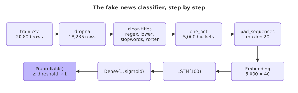
The Embedding layer in Keras lesson turned short sentences into vectors. This practical puts the same steps in front of an LSTM (long short-term memory) layer and trains it on the titles of 18,285 news articles.
Getting the fake news dataset
The data is train.csv from the Fake News competition on Kaggle (a Kaggle login is needed to download it). It has 20,800 articles with five columns: id, title, author, text and label, where 1 means unreliable and 0 reliable. The video uploads the file to Colab and predicts the label from the title alone.
import pandas as pd
df=pd.read_csv('train.csv')
df.isnull().sum()id 0 title 558 author 1957 text 39 label 0 dtype: int64
A missing title or text cannot be filled in sensibly, so the notebook drops every row with a missing value and splits the columns into features X and the label y:
###Drop Nan Values
df=df.dropna()
## Get the Independent Features

X=df.drop('label',axis=1)
## Get the Dependent features
y=df['label']
X.shape(18285, 4)
Preparing the titles
The notebook imports the Keras pieces, sets the vocabulary size to 5,000 and copies X into messages. Because dropna removed rows, the row labels now have gaps; reset_index renumbers them 0, 1, 2 and so on.
from tensorflow.keras.layers import Embedding
from tensorflow.keras.preprocessing.sequence import pad_sequences
from tensorflow.keras.models import Sequential
from tensorflow.keras.preprocessing.text import one_hot
from tensorflow.keras.layers import LSTM
from tensorflow.keras.layers import Dense
### Vocabulary size
voc_size=5000
messages=X.copy()
messages.reset_index(inplace=True)
The cleaning loop below reads messages['title'][i], which looks rows up by label, so this reset_index line has to run. Without it the loop stops at the first missing label, here with KeyError: 6. The same failure on a three-row table:
import pandas as pd

df = pd.DataFrame({"title": ["first title", None, "third title"], "label": [1, 0, 1]})
messages = df.dropna()                     # row 1 is dropped, the labels are now 0 and 2
print("index after dropna:", messages.index.tolist())
try:
    for i in range(len(messages)):
        print(messages['title'][i])
except KeyError as err:
print("KeyError:", err) # there is no row labelled 1 any moreindex after dropna: [0, 2] first title KeyError: 1
import pandas as pd

df = pd.DataFrame({"title": ["first title", None, "third title"], "label": [1, 0, 1]})
messages = df.dropna()
messages.reset_index(inplace=True)         # the labels become 0, 1 again
for i in range(len(messages)):
print(messages['title'][i])first title third title
Cleaning the titles with stemming and stopwords
The cleaning builds a list called corpus, one cleaned title per row. For each title it replaces everything except the letters a to z and A to Z with a space, lowercases the result, splits it into words, and in a list comprehension keeps the Stemming of every word that is not in the English Stopwords list. The words are joined back into one string. Lemmatization would also work, but on about 18,000 titles it takes longer than stemming.
import nltk
import re
from nltk.corpus import stopwords
nltk.download('stopwords')[nltk_data] Downloading package stopwords to /root/nltk_data... [nltk_data] Package stopwords is already up-to-date! True
### Dataset Preprocessing
from nltk.stem.porter import PorterStemmer ##stemming purpose
ps = PorterStemmer()
corpus = []
for i in range(0, len(messages)):
    review = re.sub('[^a-zA-Z]', ' ', messages['title'][i])
    review = review.lower()
    review = review.split()

    review = [ps.stem(word) for word in review if not word in stopwords.words('english')]
    review = ' '.join(review)
corpus.append(review)corpus[1]'flynn hillari clinton big woman campu breitbart'
The same loop on the first six titles of the file, with today's NLTK. The stopwords become a set built once: calling stopwords.words('english') for every word re-reads the list each time and makes the loop far slower, with the same result.
import re
from nltk.corpus import stopwords
from nltk.stem.porter import PorterStemmer

titles = [
    'House Dem Aide: We Didn’t Even See Comey’s Letter Until Jason Chaffetz Tweeted It',
    'FLYNN: Hillary Clinton, Big Woman on Campus - Breitbart',
    'Why the Truth Might Get You Fired',
    '15 Civilians Killed In Single US Airstrike Have Been Identified',
    'Iranian woman jailed for fictional unpublished story about woman stoned to death for adultery',
    'Jackie Mason: Hollywood Would Love Trump if He Bombed North Korea over Lack of Trans Bathrooms (Exclusive Video) - Breitbart',
]
ps = PorterStemmer()
stop = set(stopwords.words('english'))      # built once, not once per word
corpus = []
for title in titles:
    review = re.sub('[^a-zA-Z]', ' ', title)
    review = review.lower().split()
    review = [ps.stem(word) for word in review if word not in stop]
    corpus.append(' '.join(review))
for line in corpus:
print(line)hous dem aid even see comey letter jason chaffetz tweet flynn hillari clinton big woman campu breitbart truth might get fire civilian kill singl us airstrik identifi iranian woman jail fiction unpublish stori woman stone death adulteri jacki mason hollywood would love trump bomb north korea lack tran bathroom exclus video breitbart
The six lines match the first six entries of the notebook's saved corpus, word for word. Notice "breitbart" at the end of two of them: the outlet's name is part of the title.
Encoding and padding the titles
one_hot hashes each stemmed word into a number from 1 to 4,999. The second title, 'flynn hillari clinton big woman campu breitbart', becomes seven numbers; in this run "flynn" is 2861:
onehot_repr=[one_hot(words,voc_size)for words in corpus]
onehot_repr[1][2861, 147, 1342, 1829, 62, 4605, 721]
With 13,931 distinct stems and 4,999 buckets, most buckets hold several words, so different words share a number. Every title is then padded to 20 numbers, this time at the end:
sent_length=20
embedded_docs=pad_sequences(onehot_repr,padding='post',maxlen=sent_length)
print(embedded_docs)
embedded_docs[1][[4623 3077 4413 ... 0 0 0]
[2861 147 1342 ... 0 0 0]
[4719 1908 3457 ... 0 0 0]
...
[1998 2936 526 ... 0 0 0]
[ 983 563 4899 ... 0 0 0]
[2944 4643 913 ... 0 0 0]]
array([2861, 147, 1342, 1829, 62, 4605, 721, 0, 0, 0, 0,
0, 0, 0, 0, 0, 0, 0, 0, 0], dtype=int32)A length of 20 covers almost every title, but not all: after cleaning, the longest has 47 words, 37 titles are longer than 20 and lose their first words to the default truncating='pre', and 54 titles clean to nothing and become 20 zeros.
Building the LSTM model
The model is a Sequential stack of three layers. The Embedding layer takes the vocabulary size (5,000), the number of features per word (40) and the input length (20), so every index becomes 40 numbers. The LSTM layer has 100 units; 200 or 300 would also work, and the number is a hyperparameter. The output is one Dense unit with a sigmoid, because the label is binary, and a binary output goes with binary cross-entropy as the loss, Adam as the optimizer and accuracy as the metric. The summary reports 256,501 parameters.
## Creating model
embedding_vector_features=40 ##features representation
model=Sequential()
model.add(Embedding(voc_size,embedding_vector_features,input_length=sent_length))
model.add(LSTM(100))
model.add(Dense(1,activation='sigmoid'))
model.compile(loss='binary_crossentropy',optimizer='adam',metrics=['accuracy'])
print(model.summary())Model: "sequential_2"
_________________________________________________________________
Layer (type) Output Shape Param #
=================================================================
embedding_2 (Embedding) (None, 20, 40) 200000
lstm_2 (LSTM) (None, 100) 56400
dense_2 (Dense) (None, 1) 101
=================================================================
Total params: 256,501
Trainable params: 256,501
Non-trainable params: 0
_________________________________________________________________
NoneOn Keras 3, input_length is deprecated and one_hot no longer exists; the section on today's Keras below shows the current form of both.
The 40 numbers per word are learned by backpropagation together with the LSTM, from the binary cross-entropy of this task. The parameter counts follow from the layer sizes:
voc_size, dim, units = 5000, 40, 100
embedding = voc_size * dim                          # one 40-number row per index
lstm = 4 * (units * (units + dim) + units)          # four layers on [h(t-1), x(t)], one bias each
dense = units * 1 + 1
print("embedding:", embedding, " lstm:", lstm, " dense:", dense, " total:", embedding + lstm + dense)
print("training steps per epoch:", -(-12250 // 64)) # 12,250 training rows in batches of 64embedding: 200000 lstm: 56400 dense: 101 total: 256501 training steps per epoch: 192
Training and evaluating the model
The padded titles become NumPy arrays and are split, a third for testing (Train and test split):
import numpy as np
X_final=np.array(embedded_docs)
y_final=np.array(y)
X_final.shape,y_final.shape((18285, 20), (18285,))
from sklearn.model_selection import train_test_split
X_train, X_test, y_train, y_test = train_test_split(X_final, y_final, test_size=0.33, random_state=42)
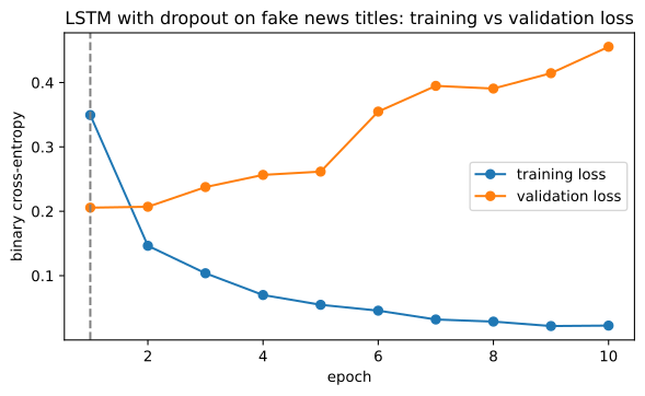
The video trains this model for 10 epochs, then adds Dropout with a rate of 0.3 after the Embedding and after the LSTM layer and trains again. The training log saved in the notebook is the run of this second model:
from tensorflow.keras.layers import Dropout
## Creating model
embedding_vector_features=40
model=Sequential()
model.add(Embedding(voc_size,embedding_vector_features,input_length=sent_length))
model.add(Dropout(0.3))
model.add(LSTM(100))
model.add(Dropout(0.3))
model.add(Dense(1,activation='sigmoid'))
model.compile(loss='binary_crossentropy',optimizer='adam',metrics=['accuracy'])### Finally Training
model.fit(X_train,y_train,validation_data=(X_test,y_test),epochs=10,batch_size=64)Epoch 1/10 192/192 [==============================] - 4s 11ms/step - loss: 0.3495 - accuracy: 0.8247 - val_loss: 0.2056 - val_accuracy: 0.9114 Epoch 2/10 192/192 [==============================] - 2s 9ms/step - loss: 0.1464 - accuracy: 0.9429 - val_loss: 0.2070 - val_accuracy: 0.9104 Epoch 3/10 192/192 [==============================] - 2s 8ms/step - loss: 0.1037 - accuracy: 0.9635 - val_loss: 0.2376 - val_accuracy: 0.9125 Epoch 4/10 192/192 [==============================] - 2s 8ms/step - loss: 0.0699 - accuracy: 0.9758 - val_loss: 0.2565 - val_accuracy: 0.9183 Epoch 5/10 192/192 [==============================] - 2s 9ms/step - loss: 0.0547 - accuracy: 0.9801 - val_loss: 0.2616 - val_accuracy: 0.9075 Epoch 6/10 192/192 [==============================] - 2s 8ms/step - loss: 0.0456 - accuracy: 0.9839 - val_loss: 0.3549 - val_accuracy: 0.9127 Epoch 7/10 192/192 [==============================] - 2s 8ms/step - loss: 0.0319 - accuracy: 0.9891 - val_loss: 0.3948 - val_accuracy: 0.8998 Epoch 8/10 192/192 [==============================] - 2s 8ms/step - loss: 0.0286 - accuracy: 0.9904 - val_loss: 0.3906 - val_accuracy: 0.9072 Epoch 9/10 192/192 [==============================] - 2s 8ms/step - loss: 0.0217 - accuracy: 0.9923 - val_loss: 0.4145 - val_accuracy: 0.9054 Epoch 10/10 192/192 [==============================] - 2s 8ms/step - loss: 0.0224 - accuracy: 0.9918 - val_loss: 0.4555 - val_accuracy: 0.9036
The predictions are probabilities; a threshold turns them into 0 or 1. The notebook uses 0.6, then prints the Confusion matrix, the accuracy and the classification report:
y_pred=model.predict(X_test)
y_pred=np.where(y_pred > 0.6, 1,0) ##AUC ROC Curve
from sklearn.metrics import confusion_matrixconfusion_matrix(y_test,y_pred)array([[3135, 284],
[ 297, 2319]])from sklearn.metrics import accuracy_score
accuracy_score(y_test,y_pred)0.903728251864126
from sklearn.metrics import classification_report
print(classification_report(y_test,y_pred)) precision recall f1-score support
0 0.91 0.92 0.92 3419
1 0.89 0.89 0.89 2616
accuracy 0.90 6035
macro avg 0.90 0.90 0.90 6035
weighted avg 0.90 0.90 0.90 6035import numpy as np
import matplotlib.pyplot as plt
# loss and val_loss copied from the saved training log above (the model with Dropout)
loss = [0.3495, 0.1464, 0.1037, 0.0699, 0.0547, 0.0456, 0.0319, 0.0286, 0.0217, 0.0224]
val_loss = [0.2056, 0.2070, 0.2376, 0.2565, 0.2616, 0.3549, 0.3948, 0.3906, 0.4145, 0.4555]
epochs = np.arange(1, 11)
best = int(np.argmin(val_loss)) + 1
print("lowest val_loss:", min(val_loss), "at epoch", best)
print("val_loss at epoch 10 is", round(val_loss[-1] / min(val_loss), 2), "times the lowest")
plt.figure(figsize=(7, 3.8))
plt.plot(epochs, loss, marker="o", label="training loss")
plt.plot(epochs, val_loss, marker="o", label="validation loss")
plt.axvline(best, color="grey", linestyle="--")
plt.xlabel("epoch")
plt.ylabel("binary cross-entropy")
plt.title("LSTM with dropout on fake news titles: training vs validation loss")
plt.legend()
plt.show()lowest val_loss: 0.2056 at epoch 1 val_loss at epoch 10 is 2.22 times the lowest
Reading the training log and the scores
- 192 steps per epoch: 12,250 training rows in batches of 64.
- Training accuracy ends at 0.9918 while validation accuracy stays near 0.90 to 0.92.
- Validation loss is lowest after epoch 1 (0.2056) and more than doubles by epoch 10: the model overfits after the first pass. Early stopping on
val_losswould keep the epoch-1 weights. - Test accuracy is 0.9037 on 6,035 titles at a threshold of 0.6, with 284 reliable titles flagged as unreliable and 297 unreliable ones missed.
- The plain LSTM, before dropout, scored 0.9084 on the same test set at a threshold of 0.5 in the video's run, with the confusion matrix [[3156, 263], [290, 2326]]: dropout did not help here.
- The validation data is the test set itself. A separate validation split (
validation_split=0.1on the training data) keeps the test score untouched by choices made while training.
Checking what the model learned
Before trusting the score, compare it with a rule that does not read the news at all. The code needs the competition's train.csv:
import numpy as np
import pandas as pd
from sklearn.model_selection import train_test_split

df = pd.read_csv('train.csv').dropna()
title = df['title'].str.lower()
named = title.str.contains('new york times') | title.str.contains('breitbart')
pred = np.where(named, 0, 1)               # names one of two outlets -> reliable, else unreliable
_, p_test, _, y_test = train_test_split(pred, df['label'].to_numpy(), test_size=0.33, random_state=42)
print((p_test == y_test).mean())
It prints 0.8966. Of the 18,285 titles, 46.8% contain "New York Times" or "Breitbart", and only 0.19% of those are labelled unreliable. The LSTM's 0.90 is little more than this rule: most of what it learned is the outlet's name at the end of the title.
Writing the model with today's Keras
import keras
from keras import layers

vectorize = layers.TextVectorization(max_tokens=5000, output_sequence_length=20)
vectorize.adapt(corpus)
X_final = vectorize(np.array(corpus))      # a real vocabulary instead of hashing

model = keras.Sequential([
    keras.Input(shape=(20,)),
    layers.Embedding(5000, 40, mask_zero=True),   # skip the padded positions
    layers.LSTM(100),
    layers.Dense(1, activation="sigmoid"),
])model.compile(loss="binary_crossentropy", optimizer="adam", metrics=["accuracy"])
stop = keras.callbacks.EarlyStopping(monitor="val_loss", patience=2, restore_best_weights=True)
model.fit(X_train, y_train, validation_split=0.1, epochs=10, batch_size=64, callbacks=[stop])one_hotis gone in Keras 3;TextVectorizationreplaces it.input_lengthis deprecated;keras.Input(shape=(20,))gives the shape.mask_zero=Truestops the LSTM from reading the trailing padding zeros.validation_splitandEarlyStoppingkeep the test set out of training decisions.
Plain LSTM vs LSTM with dropout
| Plain LSTM | With Dropout(0.3) | |
|---|---|---|
| Threshold | 0.5 | 0.6 |
| Test accuracy | 0.9084 | 0.9037 |
| Confusion matrix | [[3156, 263], [290, 2326]] | [[3135, 284], [297, 2319]] |
| Parameters | 256,501 | 256,501 (dropout adds none) |
Where you use LSTM text classification
- Moderation and spam filtering, where the order of words changes the meaning.
- Sentiment and topic labelling of reviews, tickets and posts.
- A step up from bag-of-words models such as the Spam classifier with BoW and TF-IDF, once those baselines are known.
Related
- Previous: Embedding layer in Keras
- Next: Bidirectional LSTM
- See also: Spam classifier with BoW and TF-IDF
- Add a seventh title to the cleaning example that ends in " - The New York Times" and look at what its last three stems are.
- In the curve example, find the epoch where training loss first drops below 0.05 and compare validation loss at that epoch with its lowest value.
- Change
units = 100tounits = 200in the parameter example and see how much the LSTM layer grows.
You understood something today that you didn't yesterday.