
Positional encoding
Positional encoding is a vector added to each token's embedding that tells a transformer where the token sits in the sequence, because self-attention on its own treats its input as an unordered set.
Last updated: 07 Oct, 2026 · NumPy
Every transformer layer so far, from Self-attention to the Position-wise feed-forward network, processes the tokens in parallel. Nothing in them knows which token came first.
Losing word order in parallel processing
The major advantage of the transformer is that all the word tokens are processed in parallel: x1 and x2 go into the self-attention layer at once. The drawback that comes with it is that the model lacks the sequential structure of the words, their order. Self-attention has no idea whether x1 or x2 came first.
The video's example is "lion kills tiger" and "tiger kills lion". The order changes the meaning completely, but both sentences hold the same three words, and self-attention returns the same vector for each word in both. The fix from "Attention Is All You Need" is a positional encoding vector of the same size as the embedding, made for each position and added to that word's embedding, so the sum tells the model which word sits where.
Showing that self-attention ignores order
The run uses the embeddings from the video's positional-encoding example, The = [0.1, 0.2, 0.3, 0.4], cat = [0.5, 0.6, 0.7, 0.8] and sat = [0.9, 1.0, 1.1, 1.2], in two orders, "The cat sat" and "sat cat The", and prints cat's self-attention output in both: once without and once with the sinusoidal encoding defined further down.
import numpy as np

emb = {"The": [0.1, 0.2, 0.3, 0.4], "cat": [0.5, 0.6, 0.7, 0.8], "sat": [0.9, 1.0, 1.1, 1.2]}

def self_attention(X):
    s = X @ X.T / np.sqrt(X.shape[1])
    w = np.exp(s) / np.exp(s).sum(axis=1, keepdims=True)
    return w @ X

def pe(n, d):                                      # sinusoidal positional encoding
    pos, i = np.arange(n)[:, None], np.arange(d // 2)[None, :]
    P = np.zeros((n, d))
    P[:, 0::2] = np.sin(pos / 10000 ** (2 * i / d))
    P[:, 1::2] = np.cos(pos / 10000 ** (2 * i / d))
    return P

for add_pe in (False, True):
    out = {}
    for sentence in (["The", "cat", "sat"], ["sat", "cat", "The"]):
        X = np.array([emb[w] for w in sentence])
        if add_pe:
            X = X + pe(3, 4)
        Z = self_attention(X)
        out[" ".join(sentence)] = Z[sentence.index("cat")]
    a, b = out.values()
    print("with PE   " if add_pe else "without PE", "cat in both orders:", np.round(a, 4), np.round(b, 4),
"same" if np.allclose(a, b) else "different")without PE cat in both orders: [0.6328 0.7328 0.8328 0.9328] [0.6328 0.7328 0.8328 0.9328] same with PE cat in both orders: [1.4906 0.8314 0.9036 1.9888] [1.0446 1.579 0.9247 2.0202] different
- Without positional encoding cat comes out as [0.6328, 0.7328, 0.8328, 0.9328] in both orders: reordering the input only reorders the output.
- With positional encoding cat comes out different in the two orders, although it sits at position 1 both times: its neighbours now carry different positions.
Choosing between position numbers, sinusoids and learned vectors
One simple idea is to add one more dimension to each embedding that holds the position: 1 for the first word, 2 for the second, 3 for the third. For a short text that works, but a book, a journal or a novel may have more than 100,000 words, and the position values have no upper limit. Adding such large numbers to the vectors causes problems in backpropagation, when the weights are updated.
The paper instead adds a positional encoding vector of the same size as the embedding. There are two types: sinusoidal positional encoding, the one the paper uses, and learned positional encoding. The sinusoidal one uses sine and cosine functions of different frequencies, and all its values stay between −1 and +1, however many words there are.
Here pos is the position of the token, starting at 0, dmodel is the size of the embeddings, and i is the pair index, from 0 to dmodel/2 − 1. Dimensions 2i and 2i + 1 form a pair that shares one frequency, ωi = 1/100002i/dmodel: sin goes in the even dimension and cos in the odd one. The frequency falls from pair to pair, so the wavelengths run from 2π up to 10000 · 2π.
Computing the encoding for The cat sat
The video's example has dmodel = 4, so there are two pairs. Pair i = 0 (dimensions 0 and 1) uses pos/100000/4 = pos, and pair i = 1 (dimensions 2 and 3) uses pos/100002/4 = pos/100.
- pos = 0 (The): [sin 0, cos 0, sin 0, cos 0] = [0, 1, 0, 1].
- pos = 1 (cat): [sin 1, cos 1, sin 0.01, cos 0.01] = [0.8415, 0.5403, 0.0100, 0.99995].
- pos = 2 (sat): [sin 2, cos 2, sin 0.02, cos 0.02] = [0.9093, −0.4161, 0.0200, 0.9998].
Each encoding is added to its token's embedding, number by number.
![Positional encoding for The cat sat with d_model = 4: The at position 0 has embedding [0.1, 0.2, 0.3, 0.4] plus PE [0, 1, 0, 1], giving [0.1, 1.2, 0.3, 1.4]; cat at position 1 has [0.5, 0.6, 0.7, 0.8] plus [0.8415, 0.5403, 0.0100, 0.99995], giving [1.3415, 1.1403, 0.71, 1.79995]; sat at position 2 has [0.9, 1.0, 1.1, 1.2] plus [0.9093, -0.4161, 0.0200, 0.9998], giving [1.8093, 0.5839, 1.12, 2.1998].](https://d14omfvx1qlabb.cloudfront.net/krishnaik.in/media/tutorials/nlp/7ee11ed34ce342919d34a216e15a3981.svg)
The encoding function
angle = pos / 10000 ** (2 * i / d)    # pos as a column, pair index i as a row
P[:, 0::2] = np.sin(angle)            # even dimensions 2i
P[:, 1::2] = np.cos(angle) # odd dimensions 2i + 1import numpy as np
np.set_printoptions(suppress=True)
def pe(n, d):
pos = np.arange(n)[:, None] # positions 0, 1, 2, ...
i = np.arange(d // 2)[None, :] # pair index 0 .. d/2 - 1
angle = pos / 10000 ** (2 * i / d)
P = np.zeros((n, d))
P[:, 0::2] = np.sin(angle) # even dimensions 2i
P[:, 1::2] = np.cos(angle) # odd dimensions 2i + 1
return P
E = np.array([[0.1, 0.2, 0.3, 0.4], # The (position 0)
[0.5, 0.6, 0.7, 0.8], # cat (position 1)
[0.9, 1.0, 1.1, 1.2]]) # sat (position 2)
P = pe(3, 4)
print("PE for positions 0, 1, 2 (d_model = 4):\n", np.round(P, 5))
print("embedding + PE:\n", np.round(E + P, 5))PE for positions 0, 1, 2 (d_model = 4): [[ 0. 1. 0. 1. ] [ 0.84147 0.5403 0.01 0.99995] [ 0.9093 -0.41615 0.02 0.9998 ]] embedding + PE: [[0.1 1.2 0.3 1.4 ] [1.34147 1.1403 0.71 1.79995] [1.8093 0.58385 1.12 2.1998 ]]
- The three PE rows match the hand calculation: [0, 1, 0, 1], [0.84147, 0.5403, 0.01, 0.99995] and [0.9093, −0.41615, 0.02, 0.9998].
- The sums are what self-attention receives: The [0.1, 1.2, 0.3, 1.4], cat [1.34147, 1.1403, 0.71, 1.79995] and sat [1.8093, 0.58385, 1.12, 2.1998].
- The second pair changes slowly, 0, 0.01 and 0.02 in its sin, because its frequency is 100 times lower than the first pair's.
Plotting the encoding at d_model = 512
At the paper's size, dmodel = 512, the encodings of 100 positions form a clear pattern.
import numpy as np
import matplotlib.pyplot as plt
np.set_printoptions(suppress=True)

def pe(n, d):
    pos, i = np.arange(n)[:, None], np.arange(d // 2)[None, :]
    P = np.zeros((n, d))
    P[:, 0::2] = np.sin(pos / 10000 ** (2 * i / d))
    P[:, 1::2] = np.cos(pos / 10000 ** (2 * i / d))
    return P

P = pe(100, 512)                                   # 100 positions, d_model = 512
print("PE[1, :6]  =", np.round(P[1, :6], 4))
print("PE[1, -4:] =", np.round(P[1, -4:], 4))
print("smallest and largest value:", round(P.min(), 4), round(P.max(), 4))
print("wavelengths run from", round(2 * np.pi, 4), "to", round(2 * np.pi * 10000 ** (510 / 512), 1))

fig, ax = plt.subplots(figsize=(8, 4))
im = ax.imshow(P, cmap="RdBu", aspect="auto", vmin=-1, vmax=1)
ax.set_xlabel("dimension (even = sin, odd = cos)")
ax.set_ylabel("position")
ax.set_title("Sinusoidal positional encoding, d_model = 512")
fig.colorbar(im, ax=ax)
plt.show()PE[1, :6] = [0.8415 0.5403 0.8219 0.5697 0.802 0.5974] PE[1, -4:] = [0.0001 1. 0.0001 1. ] smallest and largest value: -1.0 1.0 wavelengths run from 6.2832 to 60611.5
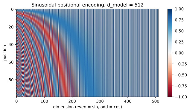
- PE[1] starts [0.8415, 0.5403, 0.8219, 0.5697, …]: sin 1 and cos 1 again, then pairs of lower frequency.
- The last pairs barely move: 0.0001 and 1.0 at position 1, so they change over thousands of positions.
- All values lie between −1.0 and 1.0, and the wavelengths run from 6.2832 (2π) to 60611.5.
- In the heat map the left columns flip quickly from row to row and the right columns are almost constant, so every position gets a different pattern.
Shifting a position is a rotation
The paper explains the choice of sin and cos pairs: for any fixed offset k, PEpos+k can be written as a linear function of PEpos. Within each pair, moving k positions rotates the (sin, cos) point by the angle k·ωi. The authors expected this to make it easy for the model to attend by relative position, and chose the sinusoid because it may let a model handle sequences longer than those seen in training.
Rotating every pair by k
out[0::2] = s * np.cos(k * w) + c * np.sin(k * w)    # the new sin
out[1::2] = c * np.cos(k * w) - s * np.sin(k * w) # the new cosimport numpy as np
def pe(n, d):
pos, i = np.arange(n)[:, None], np.arange(d // 2)[None, :]
P = np.zeros((n, d))
P[:, 0::2] = np.sin(pos / 10000 ** (2 * i / d))
P[:, 1::2] = np.cos(pos / 10000 ** (2 * i / d))
return P
d, k = 512, 3
P = pe(50, d)
w = 1 / 10000 ** (2 * np.arange(d // 2) / d) # one frequency per (sin, cos) pair
def shift(p, k): # rotate every pair by the angle k * w
s, c = p[0::2], p[1::2]
out = np.empty_like(p)
out[0::2] = s * np.cos(k * w) + c * np.sin(k * w)
out[1::2] = c * np.cos(k * w) - s * np.sin(k * w)
return out
print("PE(13) equals PE(10) rotated by k = 3:", np.allclose(shift(P[10], k), P[13]))
print("PE(40) equals PE(37) rotated by k = 3:", np.allclose(shift(P[37], k), P[40]))
print("PE5 . PE8 =", round(P[5] @ P[8], 4))
print("PE20 . PE23 =", round(P[20] @ P[23], 4))PE(13) equals PE(10) rotated by k = 3: True PE(40) equals PE(37) rotated by k = 3: True PE5 . PE8 = 211.7494 PE20 . PE23 = 211.7494
- Rotating PE(10) by k = 3 gives PE(13), and rotating PE(37) gives PE(40): the same rotation works at any position.
- PE5 · PE8 and PE20 · PE23 are both 211.7494: the dot product of two encodings depends only on how far apart they are, not on where they sit.
Sinusoidal vs learned positional encoding
| Sinusoidal | Learned | |
|---|---|---|
| Where the vectors come from | a fixed formula, no weights | a trained table, one row per position |
| Longest sequence | any length | the size of the table, fixed in training |
| In the paper | chosen; may extrapolate to longer sequences | tested; nearly identical results |
| Used by | the original transformer | BERT, GPT-2 |
Many recent large language models use neither. RoPE, the rotary position embedding of Su et al. (2021) used in LLaMA, rotates the query and key vectors by an angle that depends on the position, so the attention score itself depends on the relative position, the same rotation idea as the sinusoid's.
Where you use positional encoding
- The input of every transformer, encoder and decoder, before the first layer.
- Image patches: vision transformers add a position vector to each patch for the same reason.
- Long-context models, where the scheme (sinusoidal, learned, RoPE, ALiBi) decides how well a model handles sequences longer than those it was trained on.
Related
- Previous: Position-wise feed-forward network
- Next: Residual connections and layer normalization
- Reference: Vaswani et al., Attention Is All You Need (2017)
- Print
pe(3, 8)and check that its first two columns match the dmodel = 4 encoding. - In the order example, use
["cat", "The", "sat"]as the second sentence: without positional encoding, cat's output still does not change. - Check the rotation with
k = 7, fromP[20]toP[27].
You understood something today that you didn't yesterday.