
Backpropagation through time (BPTT)
Backpropagation through time (BPTT) is backpropagation applied to an RNN unrolled over its time steps: the gradient for each shared weight is a sum with one term per step, and each term is carried back through the chain of hidden states.
Last updated: 07 Oct, 2026 · TensorFlow 2 / Keras · NumPy
The Recurrent neural network (RNN) lesson ran the forward pass and stopped at ŷ. Training compares ŷ with the label, computes a loss and moves every weight against its gradient, as in Backpropagation and weight update. In an RNN the same weights are used at every step, and that changes how the gradient is collected.
Updating the weights with gradient descent
After the forward pass the network goes the other way, from the loss back to the inputs, and every weight it meets gets updated. The first weight on the way back is the one between the last state and the output, here wy (the w′ drawn beside the output on the board). The update rule is the gradient descent rule from the ANN sessions, with a learning rate η:
The loss is computed from ŷ, and ŷ is computed from wy, so the chain rule has two links:
Following the chain rule back through time
The input weights Wx are used at every step. The chain from the loss through ŷ to the last state h4 and into the Wx of step 4 is one path. But h4 also depends on h3, which was made with the same Wx at step 3, and h3 depends on h2, and so on. Each of these paths is a term, and the gradient is their sum:
∂⁺hk/∂Wx is the direct effect of Wx at step k only, with hk−1 held fixed. The same sum, with hk−1 in place of xk, gives the gradient for Wh. For the tanh RNN each link in the product is
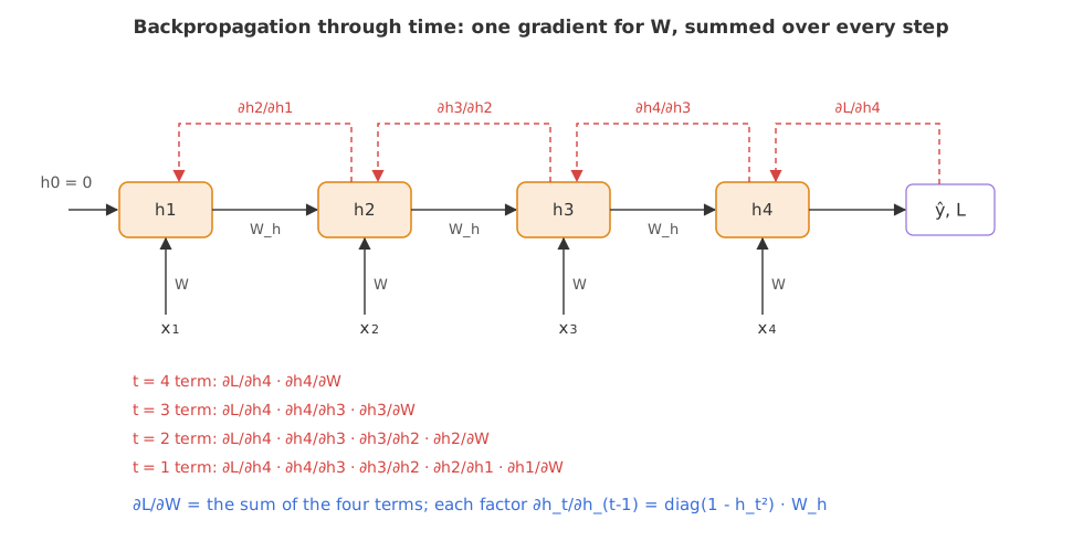
There is one Wx and one Wh for the whole sequence, so the terms from all the steps are added into one gradient and the weights get one update per training step. The chain from the loss to step 4 alone is only the first term of the sum.
Computing BPTT on "The food is very good"
The code reuses the five-word sentence and the weights of the forward-pass lesson (same seed), adds the label y = 1 and the binary cross-entropy loss, and computes every gradient by BPTT. A numerical gradient then checks the result: each weight is nudged up and down by 10⁻⁶ and the change in the loss is measured.
The forward pass that keeps every state
BPTT needs every ht, so the forward pass stores the whole list.
def forward(W_x, W_h, w_y):
    hs = [np.zeros(H)]                # h0 = 0
    for x in X:
        hs.append(np.tanh(W_x @ x + W_h @ hs[-1]))
    p = 1 / (1 + np.exp(-(w_y @ hs[-1])))
    loss = -(y * np.log(p) + (1 - y) * np.log(1 - p))   # binary cross-entropy
    return loss, p, hs
The backward loop over the steps
For a sigmoid output with cross-entropy, ∂L/∂score = ŷ − y, so ∂L/∂h5 = (ŷ − y)·wy. The loop then walks from t = 5 down to t = 1: it goes back through tanh, adds the step's term to the gradient, and multiplies by Whᵀ to reach the step before.
for t in range(T, 0, -1):
    da = dh * (1 - hs[t] ** 2)        # back through tanh at step t
    dW_x += np.outer(da, X[t - 1])    # step t's term, added to the one shared gradient
    dW_h += np.outer(da, hs[t - 1])
    dh = W_h.T @ da                   # carry the gradient back to h(t-1)
Checking against a numerical gradient
def numeric(M):                       # nudge each weight up and down by 1e-6
    g = np.zeros_like(M)
    for i in np.ndindex(M.shape):
        old = M[i]
        M[i] = old + 1e-6; up = forward(W_x, W_h, w_y)[0]
        M[i] = old - 1e-6; down = forward(W_x, W_h, w_y)[0]
        M[i] = old
        g[i] = (up - down) / 2e-6
return gimport numpy as np
rng = np.random.default_rng(42)
T, D, H = 5, 4, 3
X = rng.normal(0, 1, (T, D)) # "The food is very good", one vector per word
y = 1.0 # the label: positive
W_x = rng.normal(0, 0.5, (H, D))
W_h = rng.normal(0, 0.5, (H, H))
w_y = rng.normal(0, 0.5, H)
def forward(W_x, W_h, w_y):
hs = [np.zeros(H)] # h0 = 0
for x in X:
hs.append(np.tanh(W_x @ x + W_h @ hs[-1]))
p = 1 / (1 + np.exp(-(w_y @ hs[-1])))
loss = -(y * np.log(p) + (1 - y) * np.log(1 - p)) # binary cross-entropy
return loss, p, hs
loss, p, hs = forward(W_x, W_h, w_y)
dz = p - y # dL/dscore for a sigmoid output with cross-entropy
dw_y = dz * hs[-1]
dh = dz * w_y # dL/dh5
dW_x, dW_h, size = np.zeros_like(W_x), np.zeros_like(W_h), {}
for t in range(T, 0, -1):
da = dh * (1 - hs[t] ** 2)
dW_x += np.outer(da, X[t - 1])
dW_h += np.outer(da, hs[t - 1])
size[t] = np.linalg.norm(np.outer(da, X[t - 1]))
dh = W_h.T @ da
def numeric(M): # nudge each weight up and down by 1e-6
g = np.zeros_like(M)
for i in np.ndindex(M.shape):
old = M[i]
M[i] = old + 1e-6; up = forward(W_x, W_h, w_y)[0]
M[i] = old - 1e-6; down = forward(W_x, W_h, w_y)[0]
M[i] = old
g[i] = (up - down) / 2e-6
return g
print("loss =", round(float(loss), 4), " y_hat =", round(float(p), 4))
for name, a, M in [("w_y", dw_y, w_y), ("W_x", dW_x, W_x), ("W_h", dW_h, W_h)]:
print(f"dL/d{name}: analytic and numerical agree to 1e-8: {np.allclose(a, numeric(M), atol=1e-8)}")
last = np.outer(dz * w_y * (1 - hs[T] ** 2), X[T - 1]) # the t=5 term on its own
print("t=5 term alone vs full dL/dW_x: relative error",
round(float(np.linalg.norm(last - dW_x) / np.linalg.norm(dW_x)), 3))
print("size of each step's term (t=5..1):", [round(float(size[t]), 4) for t in range(T, 0, -1)])loss = 0.5198 y_hat = 0.5946 dL/dw_y: analytic and numerical agree to 1e-8: True dL/dW_x: analytic and numerical agree to 1e-8: True dL/dW_h: analytic and numerical agree to 1e-8: True t=5 term alone vs full dL/dW_x: relative error 0.647 size of each step's term (t=5..1): [0.1829, 0.1262, 0.0386, 0.0345, 0.0096]
What the gradient check shows
- ŷ = 0.5946 is the forward-pass lesson's P(positive); with y = 1 the loss is −ln ŷ = 0.5198.
- All three gradients agree with the numerical ones to 10⁻⁸, so the summed BPTT formula is the true derivative of the loss.
- The t = 5 term alone is 64.7% off the full ∂L/∂Wx: leaving out the earlier steps gives a different, wrong gradient.
- The terms shrink going back: 0.1829 for "good" at t = 5 down to 0.0096 for "The" at t = 1. Each step back multiplies by one more factor; Vanishing and exploding gradients in RNNs follows that product further.
import matplotlib.pyplot as plt

steps = list(range(1, T + 1))
plt.figure(figsize=(7, 3.6))
plt.bar(steps, [size[t] for t in steps], color="tab:orange")
plt.xticks(steps, ["t=1\nThe", "t=2\nfood", "t=3\nis", "t=4\nvery", "t=5\ngood"])
plt.ylabel("size of the step's term")
plt.title("Each step's share of dL/dW_x: the earlier the word, the smaller")
plt.show()
print("t=1 term / t=5 term:", round(float(size[1] / size[5]), 3))t=1 term / t=5 term: 0.053
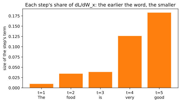
Over five words the first word's term is about a nineteenth of the last word's. Over a hundred words the early terms can all but disappear, and the network stops learning from the start of the sentence.
Truncating BPTT on long sequences
A sequence of thousands of steps needs every state kept for the backward loop. Truncated BPTT runs the backward loop over only the most recent k steps, or splits a long sequence into chunks and carries the hidden state from chunk to chunk without carrying gradients across. It trades an exact gradient for memory and speed.
BPTT vs backpropagation in a feed-forward network
| Feed-forward network | RNN with BPTT | |
|---|---|---|
| Where a weight is used | once, in its own layer | at every time step |
| Gradient of a weight | one chain-rule product | a sum of products, one per step |
| What the backward pass stores | each layer's activations | every hidden state h1 to hT |
| Depth of the longest chain | the number of layers | the length of the sequence |
Where you use BPTT
- Training any RNN, LSTM or GRU: Keras and PyTorch run BPTT automatically when you call
fitorbackward(). - Checking a hand-written gradient with the numerical check above before trusting it.
- Long time series and documents, where truncated BPTT keeps training within memory.
Related
- Previous: Types of RNN (one-to-many, many-to-one, many-to-many)
- Next: Vanishing and exploding gradients in RNNs
- See also: Chain rule of derivatives
- Change the backward loop to
for t in range(T, T - 1, -1):so only the t = 5 term is added, and see which gradient checks turn False. - Change the label to
y = 0.0and check that the gradients flip sign while the check still passes. - Make the sentence longer with
T = 10and compare the t = 1 term with the t = 10 term.
You understood something today that you didn't yesterday.