
Residual connections and layer normalization
Residual connections and layer normalization are the two operations inside every “Add & Norm” box of the transformer: the residual connection adds a sub-layer's input back to its output, and layer normalization rescales each token's vector to mean 0 and variance 1.
Last updated: 07 Oct, 2026 · NumPy
Multi-head attention and the Position-wise feed-forward network are the two sub-layers of an encoder layer. In the paper's figure each of them is followed by a yellow Add & Norm box. Those boxes are what let a stack of six encoders and six decoders train at all.
Adding the input back with a residual connection
In the encoder, the vectors that go into self-attention are also sent around it, straight to the Add & Norm box. That bypass is a residual connection, also called a skip connection. The next layer receives the sub-layer's output plus the original input, so it keeps the information about the input even after self-attention has turned it into contextual vectors.
The video gives three reasons for it, in this order:
- It addresses the vanishing gradient problem. With six encoder layers and six decoder layers, the gradient of the loss with respect to the early weights can become very small. The residual connection creates a short path for gradients to flow directly through the network, so the gradient stays large enough.
- It improves gradient flow, so training converges faster and more smoothly.
- It enables training of deeper networks. A stack of six encoders is a deep network, and the residual at every sub-layer is what makes it trainable. A layer can also learn the identity mapping (output = input) by setting its sub-layer's contribution near zero.
The derivative shows why. Backpropagation multiplies one Jacobian per layer. Without the skip, each factor is ∂F/∂x, and a product of many small factors shrinks towards zero, the Vanishing gradient problem. With the skip, each factor is I + ∂F/∂x, which stays close to the identity. The NumPy run below measures this on a 6-layer and a 24-layer stack.
Normalizing hidden values: batch norm vs layer norm
The video starts from a small table with house size (f1), number of rooms (f2) and price: 1200, 2 and 45 lakhs; 1500, 3 and 70 lakhs; 2000, 3.5 and 80 lakhs. Standard scaling turns each column into z-scores, (x − μ)/σ, with mean 0 and standard deviation 1. After the scaled inputs pass through weights, a bias and an activation, the hidden outputs Z1 and Z2 can drift to a very different distribution, so they are normalized again.
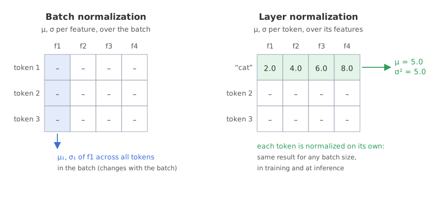
Batch normalization normalizes one column at a time: μ₁ and σ₁ are computed for Z1 over all the rows of the batch, and μ₂ and σ₂ for Z2. Layer normalization normalizes one row at a time: μ₁ and σ₁ come from the values of row 1, μ₂ and σ₂ from row 2, μ₃ and σ₃ from row 3. In a transformer each row is one token, and its 512 values are normalized on their own.
Why transformers use layer normalization
Batch statistics depend on the other sentences in the batch. With small batches they are noisy; with sentences of different lengths, the padded positions would leak into them; and at inference, when a single sentence arrives, batch norm has to fall back on running averages saved during training. Layer normalization (Ba, Kiros and Hinton, 2016) uses only the token's own dmodel = 512 features, so it gives the same result for any batch size and behaves the same in training and at inference.
Computing layer normalization for the token cat
The worked example takes one token, “cat” = [2.0, 4.0, 6.0, 8.0], with the scale γ = [1.0, 1.0, 1.0, 1.0] and the shift β = [0.0, 0.0, 0.0, 0.0]. Together γ and β are the scale and shift parameters.
- Mean: μ = ¼(2.0 + 4.0 + 6.0 + 8.0) = 20.0/4 = 5.0.
- Variance: σ² = ¼[(2.0 − 5.0)² + (4.0 − 5.0)² + (6.0 − 5.0)² + (8.0 − 5.0)²] = ¼(9 + 1 + 1 + 9) = 5.0. Layer normalization divides by N = 4, not N − 1.
- Normalize: x̂ᵢ = (xᵢ − μ)/√(σ² + ε) with ε = 1e-5 to avoid division by zero. √(5.0 + 0.00001) = 2.23607, so x̂ = [−1.3416, −0.4472, 0.4472, 1.3416].
- Scale and shift: yᵢ = γᵢx̂ᵢ + βᵢ. With γ all ones and β all zeros, y is the same vector, [−1.3416, −0.4472, 0.4472, 1.3416].
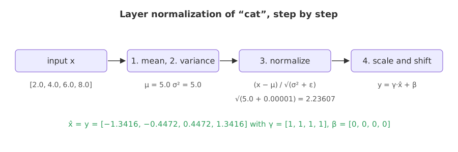
γ and β are vectors with one value per feature (512 each in the paper's model), learned by backpropagation. Starting them at ones and zeros is the default of layer-norm implementations such as PyTorch's nn.LayerNorm; the Transformer paper does not specify it. They answer the video's question “is it compulsory that we always normalize?”: the network always computes x̂, but γ and β can move the output to whatever scale and centre helps. For one token, setting γ = √(σ² + ε) and β = μ gives back the original input, so the network is never forced to keep the normalized scale.
Placing Add & Norm: post-norm vs pre-norm
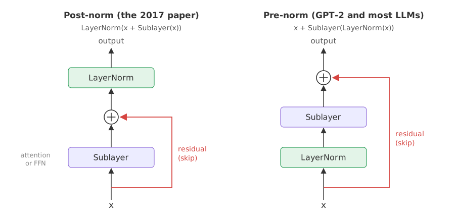
In the 2017 paper the residual is added to the output of the sub-layer, after the attention's output projection, and the sum is normalized. Dropout with rate 0.1 is applied to the sub-layer output before the add. This order is called post-norm. GPT-2 and most later large language models move the normalization to the start of each sub-layer, pre-norm, which leaves the skip path as a clean identity from the first layer to the last and trains very deep stacks more stably.
Layer normalization of cat in NumPy
The four steps from the board, with eps inside the square root. The last line sets γ and β to the token's own standard deviation and mean to show that they can undo the normalization.
import numpy as np

cat = np.array([2.0, 4.0, 6.0, 8.0])          # the token "cat" from the board
gamma = np.ones(4)                             # learned scale, starts at 1
beta = np.zeros(4)                             # learned shift, starts at 0
eps = 1e-5

mu = cat.mean()                                # step 1: mean
var = ((cat - mu) ** 2).mean()                 # step 2: variance, divided by N
x_hat = (cat - mu) / np.sqrt(var + eps)        # step 3: normalise
y = gamma * x_hat + beta                       # step 4: scale and shift

print("mean:", mu, " variance:", var, " sqrt(var + eps):", round(np.sqrt(var + eps), 5))
print("x_hat:", np.round(x_hat, 4))
print("y:    ", np.round(y, 4))
print("mean of y:", round(y.mean(), 6) + 0.0, " variance of y:", round(y.var(), 6))

# gamma and beta can undo the normalisation
y_back = np.sqrt(var + eps) * x_hat + mu
print("gamma = sqrt(var + eps), beta = mean gives back:", np.round(y_back, 4))mean: 5.0 variance: 5.0 sqrt(var + eps): 2.23607 x_hat: [-1.3416 -0.4472 0.4472 1.3416] y: [-1.3416 -0.4472 0.4472 1.3416] mean of y: 0.0 variance of y: 0.999998 gamma = sqrt(var + eps), beta = mean gives back: [2. 4. 6. 8.]
What the normalized cat vector shows
- Mean 5.0 and variance 5.0 match the board; √(5.0 + 1e-5) prints as 2.23607.
- x̂ = [−1.3416, −0.4472, 0.4472, 1.3416]: the values the board rounds to −1.34, −0.45, 0.45 and 1.34.
- y equals x̂ because γ is all ones and β all zeros.
- The variance of y is 0.999998, not exactly 1, because ε sits under the square root.
- γ = √(σ² + ε), β = μ brings back [2, 4, 6, 8]: the learnable pair can undo the normalization of this token.
Normalizing the house table both ways
The same NumPy code with axis=0 is batch normalization (each column over the three houses) and with axis=1 is layer normalization (each house over its three features). Both use the population standard deviation, np.std's default.
import numpy as np

# rows = 3 houses (samples), columns = size, rooms, price
H = np.array([[1200, 2.0, 45], [1500, 3.0, 70], [2000, 3.5, 80]])

bn = (H - H.mean(axis=0)) / H.std(axis=0)      # batch norm: each column over the batch
ln = (H - H.mean(axis=1, keepdims=True)) / H.std(axis=1, keepdims=True)  # layer norm: each row

print("batch norm (per column):\n", np.round(bn, 4))
print("column means:", np.round(bn.mean(axis=0), 4) + 0.0, " column stds:", np.round(bn.std(axis=0), 4))
print("layer norm (per row):\n", np.round(ln, 4))
print("row means:", np.round(ln.mean(axis=1), 4) + 0.0, " row stds:", np.round(ln.std(axis=1), 4))batch norm (per column): [[-1.1112 -1.3363 -1.3587] [-0.202 0.2673 0.3397] [ 1.3132 1.069 1.019 ]] column means: [0. 0. 0.] column stds: [1. 1. 1.] layer norm (per row): [[ 1.4135 -0.7455 -0.668 ] [ 1.4131 -0.7551 -0.658 ] [ 1.4134 -0.7481 -0.6653]] row means: [0. 0. 0.] row stds: [1. 1. 1.]
- Batch norm gives each column mean 0 and standard deviation 1: house size becomes −1.1112, −0.2020 and 1.3132, the z-scores of 1200, 1500 and 2000.
- Layer norm gives each row mean 0 and standard deviation 1, but here it mixes square feet with rooms and lakhs, so every house looks the same: about 1.41, −0.75, −0.66. Layer norm suits token embeddings, where all 512 numbers describe the same token, not a table of unrelated units.
Measuring the gradient through a residual stack
A stack of linear layers with small random weights, y = Wx, against the same stack with skips, y = x + Wx. The gradient that arrives at the top (a vector of ones, size 2.83) is carried down by multiplying with each layer's Jacobian.
import numpy as np

rng = np.random.default_rng(42)
d = 8
g_top = np.ones(d)                                 # gradient arriving at the top layer

for n_layers in (6, 24):
    Ws = [rng.normal(0, 0.1, (d, d)) for _ in range(n_layers)]
    g_plain, g_resid = g_top.copy(), g_top.copy()
    for W in reversed(Ws):
        g_plain = W.T @ g_plain                    # y = W x        -> dy/dx = W
        g_resid = (np.eye(d) + W).T @ g_resid      # y = x + W x    -> dy/dx = I + W
    print(f"{n_layers} layers: gradient size without residual {np.linalg.norm(g_plain):.2e}, "
f"with residual {np.linalg.norm(g_resid):.2f}")6 layers: gradient size without residual 8.62e-04, with residual 3.31 24 layers: gradient size without residual 6.86e-14, with residual 2.79
- Without residuals the gradient shrinks to 8.62e-04 after 6 layers and 6.86e-14 after 24: the early layers would learn almost nothing.
- With residuals it stays at 3.31 and 2.79, close to the 2.83 it started with, because every factor is I + W instead of W.
Batch normalization vs layer normalization
| Batch normalization | Layer normalization | |
|---|---|---|
| Statistics over | one feature, across the batch | one token, across its features |
| Depends on batch size | yes; noisy for small batches | no |
| Training vs inference | running averages at inference | the same computation |
| Padding in sequences | padded positions enter the statistics | each token on its own |
| Learnable parameters | γ, β per feature | γ, β per feature (512 in the paper) |
| Typical home | CNNs on images | transformers, RNNs |
Where you use residual connections and layer normalization
- Every transformer layer: two Add & Norm boxes in each encoder layer, three in each decoder layer.
- Large language models: pre-norm residual blocks, often with RMSNorm, a layer norm that skips the mean subtraction and β.
- Deep CNNs: ResNet introduced residual connections for image models with 100+ layers.
ddof=1) turns the cat vector into [−1.1619, −0.3873, 0.3873, 1.1619]. And leaving out ε makes any constant vector, such as an all-zero padding row, divide 0 by 0 and return NaN.Related
- Previous: Positional encoding
- Next: Transformer encoder
- See also: Vanishing gradient problem
- Reference: Layer Normalization (Ba, Kiros and Hinton, 2016)
- Change
catto[2.0, 4.0, 6.0, 80.0]and see how one large value pulls the other three normalized values together. - Set
gamma = np.full(4, 2.0)andbeta = np.full(4, 1.0): predict y before running it. - In the residual stack, raise the weight scale from
0.1to0.5and watch the plain gradient explode instead of vanish.
Slow is fine. Stopping is the only problem.