
Scaled dot-product attention
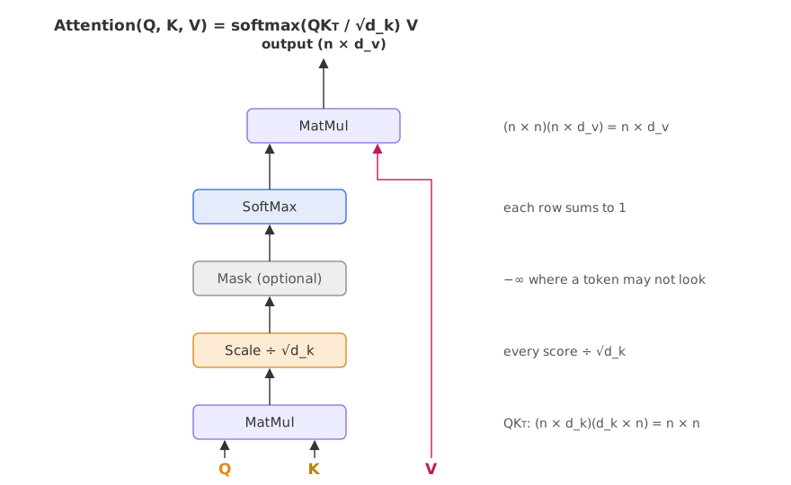
Scaled dot-product attention is the attention function of the transformer, softmax(QKT/√dk)V, which scores every query against every key with a dot product, divides the scores by the square root of the key size dk, and uses the softmax of the result to weight the values.
Last updated: 07 Oct, 2026 · NumPy
The Self-attention lesson divided its scores by 2 without saying why. Scaled dot-product attention is the function behind it. Self-attention is one use of it, where Q, K and V come from the same sequence; cross-attention, with queries from the decoder, is another.
Writing attention as matrix products
For n tokens, Q and K are n × dk matrices and V is n × dv. QKT is n × n: row i holds query i against every key. The scale and the softmax keep that shape, and multiplying by V gives n × dv, one output vector per token. The paper uses dk = dv = 64 per head. The optional mask, used in the decoder, sets the scores a token may not see to −∞ before the softmax, which makes their weights 0 (Masked self-attention).
Seeing softmax saturate without scaling
The video's example has one query and two keys: q = [2, 3, 4, 1], k₁ = [1, 0, 1, 0] and k₂ = [0, 1, 0, 1]. Without scaling, the dot products are q·k₁ = 2×1 + 3×0 + 4×1 + 1×0 = 6 and q·k₂ = 2×0 + 3×1 + 4×0 + 1×1 = 4. The softmax of the two scores is:
Most of the attention weight goes to the first key and very little to the second. Larger scores make it worse: softmax([10, 1]) is [0.99988, 0.00012], with nearly all the weight on one token. This is softmax saturation. Dividing by √dk = √4 = 2 turns [6, 4] into [3, 2], and softmax([3, 2]) = [0.7311, 0.2689], a more balanced split.
Why saturation stops learning
The paper gives the reason for the scale: for large dk the dot products grow large, "pushing the softmax function into regions where it has extremely small gradients". The gradient of a softmax output with respect to its inputs is:
When one pi is close to 1 and the others close to 0, every term is close to 0, so almost no gradient flows back to the queries and keys. It is a vanishing gradient, the problem of the Vanishing gradient problem lesson in the deep learning course. The example measures the largest gradient entry in the three cases.
Softmax and its gradient
p = softmax(z)
J = np.diag(p) - np.outer(p, p)     # J[i, j] = p_i (delta_ij - p_j)
print(np.abs(J).max()) # the largest gradient entryimport numpy as np
import matplotlib.pyplot as plt
def softmax(z):
e = np.exp(z - np.max(z))
return e / e.sum()
q = np.array([2, 3, 4, 1])
k1, k2 = np.array([1, 0, 1, 0]), np.array([0, 1, 0, 1])
raw = np.array([q @ k1, q @ k2], float) # 6 and 4
cases = {"[6, 4] unscaled": raw, "[3, 2] scaled by 2": raw / np.sqrt(4), "[10, 1]": np.array([10.0, 1.0])}
for name, z in cases.items():
p = softmax(z)
J = np.diag(p) - np.outer(p, p) # softmax gradient: dp_i/dz_j = p_i(delta_ij - p_j)
print(f"{name:<19} softmax = [{p[0]:.5f}, {p[1]:.5f}] largest gradient = {np.abs(J).max():.6f}")
fig, ax = plt.subplots(figsize=(7, 3.6))
for i, (name, z) in enumerate(cases.items()):
p = softmax(z)
ax.bar([i - 0.18, i + 0.18], p, width=0.34, color=["#e08a1e", "#3a6fd8"])
for x, v in zip([i - 0.18, i + 0.18], p):
ax.text(x, v + 0.02, f"{v:.4f}", ha="center", fontsize=9)
ax.set_xticks(range(3), list(cases))
ax.set_ylim(0, 1.12)
ax.set_ylabel("attention weight")
ax.set_title("Softmax of two scores: first key (orange), second key (blue)")
plt.show()[6, 4] unscaled softmax = [0.88080, 0.11920] largest gradient = 0.104994 [3, 2] scaled by 2 softmax = [0.73106, 0.26894] largest gradient = 0.196612 [10, 1] softmax = [0.99988, 0.00012] largest gradient = 0.000123
![Bar pairs of softmax weights: unscaled [6, 4] gives 0.8808 and 0.1192, scaled [3, 2] gives 0.7311 and 0.2689, and [10, 1] gives 0.9999 and 0.0001.](https://d14omfvx1qlabb.cloudfront.net/krishnaik.in/media/tutorials/nlp/4f03b4f236f74c20a0e3bb55189f2387.svg)
What the three softmax runs show
- Unscaled [6, 4] gives [0.88080, 0.11920] and a largest gradient of 0.104994.
- Scaled [3, 2] gives [0.73106, 0.26894] and a largest gradient of 0.196612, almost twice the signal for learning.
- [10, 1] gives [0.99988, 0.00012] and a largest gradient of 0.000123: the softmax is saturated and the scores barely learn.
Why the divisor is √d_k
Suppose the components of q and k are independent with mean 0 and variance 1. Then q·k = Σ qiki has mean 0 and variance dk (footnote 4 of the paper), so its typical size grows like √dk. Dividing by √dk brings the variance back to 1 whatever the size of the vectors. The simulation draws 100,000 random pairs for three key sizes.
import numpy as np

rng = np.random.default_rng(42)
for d_k in (4, 64, 512):
    q = rng.normal(size=(100_000, d_k))          # components with mean 0, variance 1
    k = rng.normal(size=(100_000, d_k))
    dots = (q * k).sum(axis=1)                   # 100,000 dot products q . k
print(f"d_k = {d_k:>3}: var(q.k) = {dots.var():7.2f} var(q.k / sqrt(d_k)) = {(dots / np.sqrt(d_k)).var():.3f}")d_k = 4: var(q.k) = 4.03 var(q.k / sqrt(d_k)) = 1.007 d_k = 64: var(q.k) = 63.20 var(q.k / sqrt(d_k)) = 0.988 d_k = 512: var(q.k) = 510.75 var(q.k / sqrt(d_k)) = 0.998
- The raw variance grows with dk: 4.03, 63.20 and 510.75 for dk = 4, 64 and 512.
- After dividing by √dk it stays near 1: 1.007, 0.988 and 0.998.
- At dk = 64, the paper's head size, unscaled scores would spread about 8 times wider, deep into the saturated region.
Computing the full attention matrix
As a function, scaled dot-product attention takes a few lines. The run uses one head's size, dk = dv = 64, for 3, 512 and 4096 tokens.
import numpy as np

def scaled_dot_product_attention(Q, K, V):
    d_k = K.shape[-1]
    scores = Q @ K.T / np.sqrt(d_k)                          # (n, n)
    weights = np.exp(scores - scores.max(axis=1, keepdims=True))
    weights /= weights.sum(axis=1, keepdims=True)            # softmax over the keys
    return weights @ V, weights

rng = np.random.default_rng(42)
for n in (3, 512, 4096):
    Q, K, V = (rng.normal(size=(n, 64)) for _ in range(3))  # one head: d_k = d_v = 64
    out, w = scaled_dot_product_attention(Q, K, V)
    print(f"n = {n:>4}: output {out.shape}, weights {w.shape} = {w.size:,} scores, "
f"{w.nbytes:,} bytes, rows sum to 1: {np.allclose(w.sum(1), 1)}")n = 3: output (3, 64), weights (3, 3) = 9 scores, 72 bytes, rows sum to 1: True n = 512: output (512, 64), weights (512, 512) = 262,144 scores, 2,097,152 bytes, rows sum to 1: True n = 4096: output (4096, 64), weights (4096, 4096) = 16,777,216 scores, 134,217,728 bytes, rows sum to 1: True
- The output has one 64-number row per token: (3, 64), (512, 64) and (4096, 64).
- The weight matrix is n × n: 9, 262,144 and 16,777,216 scores. Eight times the tokens gives 64 times the scores.
- At 4096 tokens one head's weights take 134,217,728 bytes in float64, for one layer. This n² growth is why long inputs are expensive for transformers.
Dot-product vs additive attention
| Scaled dot-product | Additive (Bahdanau) | |
|---|---|---|
| Score | q·k / √d_k | vᵀ tanh(Wq + Uk) |
| Extra weights in the score | none | W, U and v |
| Speed | one matrix product, fast on GPUs | a small network for every query-key pair |
| Large d_k | needs the √d_k scale | works without a scale |
Where you use scaled dot-product attention
- Every attention layer of a transformer: encoder self-attention, masked decoder self-attention and cross-attention.
- Inside each head of multi-head attention, with dk = 64 in the paper.
- Fast attention kernels such as FlashAttention compute the same function without storing the whole n × n matrix.
Related
- Previous: Self-attention
- Next: Multi-head attention
- See also: Softmax
- Reference: Vaswani et al., Attention Is All You Need (2017)
- Change q to
[4, 6, 8, 2], twice as large, and compare the unscaled softmax with [0.88, 0.12]. - Add
2048to the key sizes in the variance simulation. - In the attention function, set
scores[:, 1:] = -np.infbefore the softmax and run n = 3: every token now attends only to token 0.
This is what real progress feels like.