Vanishing gradient problem
The vanishing gradient problem is a training failure of deep networks in which the gradient shrinks as it travels back through many layers, so the weights near the input barely change.
Last updated: 05 Oct, 2026 · NumPy
The Chain rule of derivatives lesson multiplied one factor per layer to reach a weight. In a deep network the chain is long, and when every factor is small the product is tiny. The video calls this a super important interview question.
Writing the chain for a deep sigmoid network
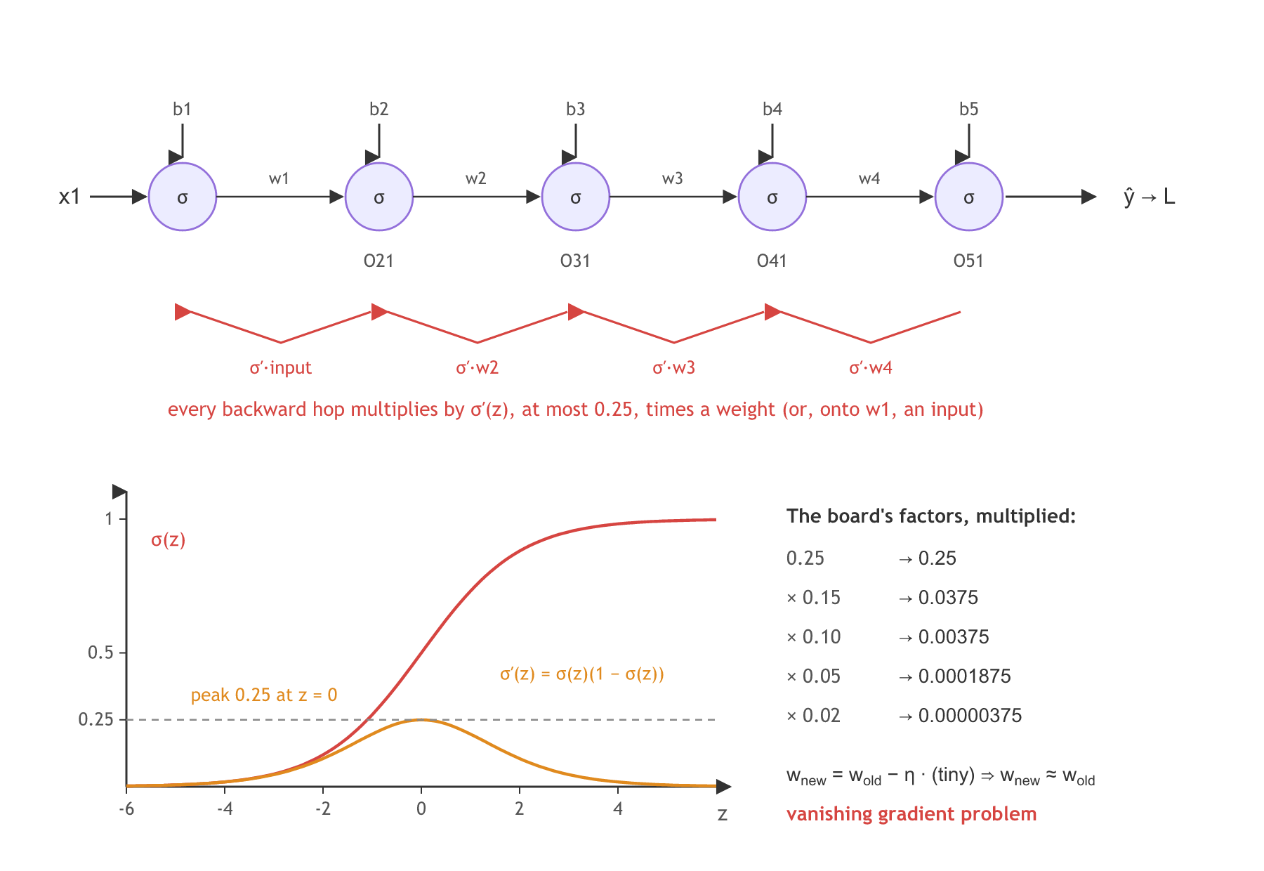
The video's network is a chain: x1 goes into five sigmoid neurons in a row, joined by weights w1 to w4, with a bias b1 to b5 into each neuron. The outputs are O21, O31, O41 and O51, then ŷ and the loss L = ½(y − ŷ)², the mean squared error for one record. To update w1, the chain runs back through every neuron:
The board writes ∂L/∂W1_new in this derivative; the slope is taken at the weight the forward pass used, so it is ∂L/∂w1_old.
Bounding the sigmoid derivative by 0.25
Every neuron here uses sigmoid, σ(z) = 1/(1 + e^(−z)); the video says it as "1 plus e to the power of minus x", leaving out the "1 over". Sigmoid outputs a value between 0 and 1 (a 0.5 threshold turns that into class 0 or 1). Its derivative, σ′(z) = σ(z)(1 − σ(z)), peaks at 0.25 at z = 0 and falls toward 0 on both sides. The board writes the bound as 0 ≤ σ(y) ≤ 0.25; it belongs to the derivative:
Each hop back in the chain goes through one sigmoid neuron. With O51 = σ(O41·w4 + b5), the hop is ∂O51/∂O41 = σ′(z)·w4. The video counts only the σ′ part; with the weight included, each hop is at most 0.25·|w|. So the gradient shrinks at every hop whenever |w| is below 4, which holds for the usual small starting weights.
Multiplying the board's small factors
The board picks example factors that keep shrinking down the chain, 0.25, 0.15, 0.10, 0.05 and 0.02, and multiplies them:
import numpy as np

factors = np.array([0.25, 0.15, 0.10, 0.05, 0.02])   # the board's example factors
print("running product:", np.cumprod(factors))
print("final:", f"{factors.prod():.2e}")running product: [2.500e-01 3.750e-02 3.750e-03 1.875e-04 3.750e-06] final: 3.75e-06
The board shows a + between 0.10 and 0.05; every step of the chain is a multiplication. The product is 3.75 × 10⁻⁶. Put it into the update rule, with a learning rate that is a small number too:
The weights hardly change, so the network stops learning. That is the vanishing gradient problem, and the video's fix is to use another activation function: tanh, ReLU, Leaky ReLU and PReLU in the next lessons. The layers nearest the input collect the most small factors, so they learn the slowest.
Measuring the gradient layer by layer in NumPy
The board's factors are examples. A real network can be measured: 10 sigmoid layers of 16 neurons with random weights, one forward pass, then the backward pass layer by layer, printing the size of each layer's weight gradient.
A 10-layer sigmoid network
import numpy as np
rng = np.random.default_rng(0)

def sigmoid(z):
    return 1 / (1 + np.exp(-z))

layers, width = 10, 16
Ws = [rng.normal(0, 1, (width, width)) for _ in range(layers)]
x = rng.normal(0, 1, width)
The forward pass, keeping each layer's output
outs = [x]
for W in Ws:
    outs.append(sigmoid(W @ outs[-1]))   # each layer's output, input side first
The backward pass, one hop per layer
Each hop multiplies by σ′(z), written with the layer's output as O(1 − O), and then by the weights. The weight gradient of a layer is its incoming gradient times its input.
g = outs[-1] - 1.0                 # dL/dO at the top, for L = 0.5 * sum((O - 1) ** 2)
norms = []
for W, O, O_in in zip(reversed(Ws), reversed(outs[1:]), reversed(outs[:-1])):
    g = g * O * (1 - O)            # times sigmoid'(z)
    norms.append(np.linalg.norm(np.outer(g, O_in)))   # size of this layer's weight gradient
    g = W.T @ g                    # times the weights: one hop back
norms = norms[::-1]                # layer 1 (input side) first
Gradient size per layer in a 10-layer sigmoid network
import matplotlib.pyplot as plt

for i, n in enumerate(norms, start=1):
    print(f"layer {i:2d}: gradient size {n:.2e}")
print(f"last layer / first layer: {norms[-1] / norms[0]:,.0f} times larger")

plt.figure(figsize=(7, 3.6))
plt.bar(range(1, layers + 1), norms, color="tab:orange")
plt.yscale("log")
plt.title("Weight-gradient size per layer, 10 sigmoid layers")
plt.xlabel("layer (1 = next to the input)")
plt.ylabel("gradient size (log scale)")
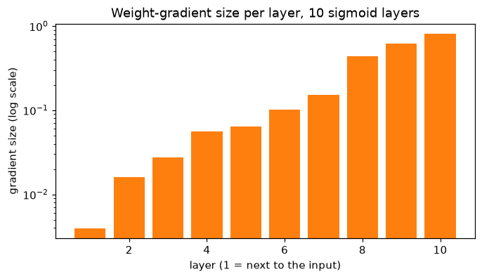
plt.show()layer 1: gradient size 3.96e-03 layer 2: gradient size 1.60e-02 layer 3: gradient size 2.76e-02 layer 4: gradient size 5.60e-02 layer 5: gradient size 6.41e-02 layer 6: gradient size 1.02e-01 layer 7: gradient size 1.53e-01 layer 8: gradient size 4.40e-01 layer 9: gradient size 6.24e-01 layer 10: gradient size 8.19e-01 last layer / first layer: 207 times larger
What the per-layer gradients show
- The gradient grows from layer 1 to layer 10: read from the output back, it shrinks at almost every hop, as the chain predicted.
- The last layer's gradient is 207 times the first layer's: with one learning rate for all layers, layer 10 moves and layer 1 stays almost where it started.
- Nothing is wrong with the code: the sigmoid derivative's 0.25 ceiling and the weights do this on their own, which is why deep networks moved to other activations.
Exploding gradients, the mirror case
The same product can also grow. If each hop factor σ′(z)·w is above 1, the gradient gets larger at every layer back: an exploding gradient. The updates become huge, the loss jumps around, and it can overflow to nan.
The run below holds every neuron at z = 0 (σ′ = 0.25) and sets every weight to w, so each hop multiplies by exactly 0.25·w:
import numpy as np

def gradient_after(w, layers=10):
    O, g = 0.5, 1.0
    for _ in range(layers):
        z = w * O - w * 0.5        # the bias -w/2 keeps z at 0
        O = 1 / (1 + np.exp(-z))   # so every output stays 0.5
        g = g * O * (1 - O) * w    # one hop back: sigmoid'(z) * w
    return g

for w in [1, 4, 8]:
print(f"w = {w}: hop factor {0.25 * w:.2f}, gradient after 10 layers {gradient_after(w):.2e}")w = 1: hop factor 0.25, gradient after 10 layers 9.54e-07 w = 4: hop factor 1.00, gradient after 10 layers 1.00e+00 w = 8: hop factor 2.00, gradient after 10 layers 1.02e+03
- w = 1: each hop is 0.25 and ten hops give 9.54 × 10⁻⁷, a vanishing gradient.
- w = 4: each hop is exactly 1 and the gradient keeps its size.
- w = 8: each hop is 2 and ten hops give 1024, an exploding gradient.
Large weights rarely rescue a sigmoid network: they push z far from 0, where σ′ is close to 0. The usual fixes are activations whose derivative is 1 for positive inputs (ReLU and its variants), starting weights scaled to the layer size (Weight initialization), and, for exploding gradients, clipping the gradient's size (Keras optimizers take a clipnorm argument).
Vanishing vs exploding gradients
| Vanishing gradient | Exploding gradient | |
|---|---|---|
| Hop factor σ′(z)·w | below 1 | above 1 |
| Gradient near the input | tiny | huge |
| What you see | early layers stop learning, loss stalls | loss jumps or becomes nan |
| In the run | w = 1: 9.54e-07 after 10 layers | w = 8: 1.02e+03 after 10 layers |
| Usual fixes | ReLU family, weight initialization | gradient clipping, weight initialization |
Where you use the vanishing gradient idea
- Interviews: "what is the vanishing gradient problem and how do you fix it" is the question the video flags; the answer is the chain of σ′(z)·w factors and a different activation.
- Choosing activations: sigmoid and tanh stay out of the hidden layers of deep networks for this reason.
- Debugging training: printing gradient sizes per layer, as the run did, shows whether the first layers are learning at all.
Related
- Previous: Chain rule of derivatives
- Next: Activation functions
- Set
layers = 20in the 10-layer network. How much smaller does the first layer's gradient get? - Start the weights smaller,
rng.normal(0, 0.1, (width, width)). Does the gradient vanish faster or slower? - Run
gradient_after(4.5)andgradient_after(3.5). Which one explodes?
Every expert started right here.