Backpropagation and weight update
Backpropagation is the backward pass of a neural network that sends the error back through the layers and updates every weight with the rule w_new = w_old − η · ∂L/∂w_old.
Last updated: 05 Oct, 2026 · NumPy
The Forward propagation lesson pushed one student (IQ 95, 4 study hours, 4 play hours) through a 3-1-1 network and got ŷ = 0.5113 for a true label of 1: an error of 0.4887 (the notes round it to 0.49), or 0.2388 when squared. Forward propagation only measures that error. Backpropagation is the half of training that reduces it, by changing the weights w1, w2, w3, w4 and the biases.
Writing the weight update formula
In the backward pass every weight gets a new value computed from its old one. The video writes one generic formula for all of them:
- w_old is the weight the forward pass used.
- η (eta) is the learning rate, a small number such as 0.01 or 0.001.
- ∂L/∂w_old is the derivative of the loss with respect to that weight: its slope, how much the loss changes when the weight changes a little.
This is the same rule that updates the coefficients of linear regression in Gradient descent. Plot the loss against one weight and you get a U-shaped curve. Its lowest point is the global minimum, the weight value with the smallest loss, and every update should move the weight toward it. The video calls this curve "gradient descent"; the curve itself is the loss function, and gradient descent is the walk down it that the update rule takes.
Reading the slope's sign on the loss curve
The video's picture is an inverted mountain: the loss surface is a bowl, and training has to walk down to its bottom. At the current weight, draw a tangent line to the curve. Its slope is ∂L/∂w, and its sign tells the weight which way to move.
- The right end of the tangent points downwards: a negative slope. The point sits on the left wall, so the weight must grow to reach the minimum. The rule gives w_new = w_old − η(−ve) = w_old + η(+ve), so w_new > w_old.
- The right end points upwards: a positive slope. The point sits on the right wall, so the weight must shrink. The rule gives w_new = w_old − η(+ve), so w_new < w_old.
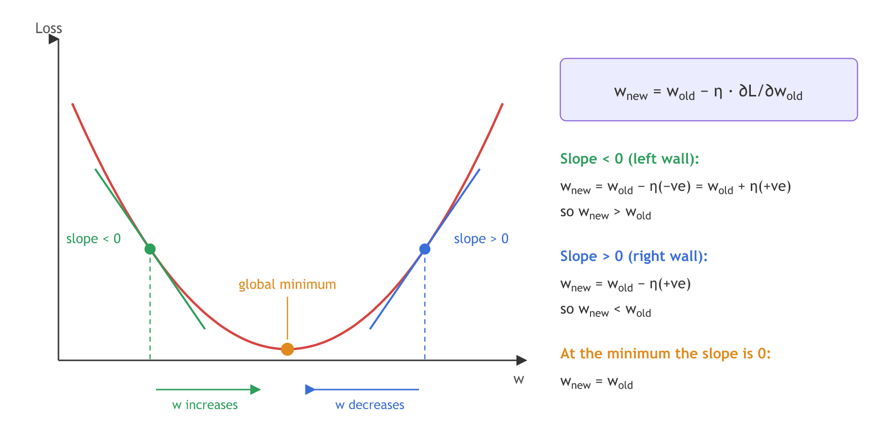
The board writes the results as w_new >> w_old and w_new << w_old. Each update is a small step, so the right signs are > and <. The notes add a third case: at the global minimum the slope is 0, so w_new = w_old and the weight stops moving.
Choosing the learning rate η
The learning rate sets the size of each step down the bowl. A small η moves slowly but steadily into the global minimum. A large η makes the weight jump from one wall to the other, and it may never settle at the minimum. The video's usual values are 0.001 and 0.01.
The run below takes 12 steps on the loss (w − 5)² + 1 from w = 1 with three learning rates.
import numpy as np
import matplotlib.pyplot as plt

def L(w):
    return (w - 5) ** 2 + 1        # a U-shaped loss, minimum at w = 5

def slope(w):
    return 2 * (w - 5)             # its derivative

plt.figure(figsize=(9, 4))
for i, eta in enumerate([0.05, 0.9, 1.05]):
    ws = [1.0]                     # start on the left wall
    for _ in range(12):
        ws.append(ws[-1] - eta * slope(ws[-1]))
    ws = np.array(ws)
    print(f"eta={eta}: w after 12 steps = {ws[-1]:.3f}")
    plt.subplot(1, 3, i + 1)
    grid = np.linspace(-2, 12, 200)
    plt.plot(grid, L(grid), color="red")
    plt.plot(ws, L(ws), "o-", color="green", markersize=4)
    plt.ylim(0, 60)
    plt.title(f"eta = {eta}")
    plt.xlabel("w")
plt.tight_layout()
plt.show()eta=0.05: w after 12 steps = 3.870 eta=0.9: w after 12 steps = 4.725 eta=1.05: w after 12 steps = -7.554
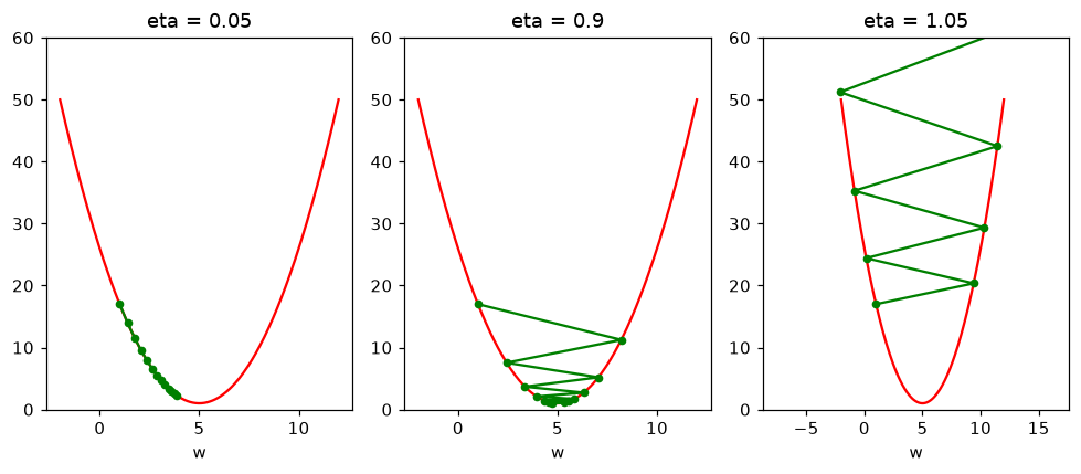
- η = 0.05 moves in the right direction every time but is still short of 5 after 12 steps: slow and steady.
- η = 0.9 overshoots to the other wall on every step and zig-zags in toward 5.
- η = 1.05 overshoots by more than it gains, so each jump lands further away: the weight never reaches the minimum.
Taking one backward step on the forward pass
Now the rule on the network from the forward propagation lesson. For one record the loss here is L = ½(y − ŷ)², the half squared error the video writes for its deep network in the vanishing gradient example; the ½ makes the derivative a clean ŷ − y.
The slope of w4 can be measured without any calculus: nudge w4 up and down by a tiny amount h, and divide the change in loss by the change in w4. The next lesson gets the same number exactly with the chain rule.
The forward pass from the board
The network, its inputs and its starting weights, written so that the loss can be computed for any choice of weights:
import numpy as np

def sigmoid(z):
    return 1 / (1 + np.exp(-z))

x = np.array([95, 4, 4])           # IQ, study hours, play hours
y = 1                              # the student passed
w = np.array([0.01, 0.02, 0.03])   # w1, w2, w3
b1, w4, b2 = 0.001, 0.02, 0.03

def loss(w, b1, w4, b2):
    O1 = sigmoid(x @ w + b1)        # hidden neuron
    y_hat = sigmoid(O1 * w4 + b2)   # output neuron
    return 0.5 * (y - y_hat) ** 2
Measuring the slope of w4
The loss a little to the right minus the loss a little to the left, divided by the distance between them:
h = 1e-6                           # a tiny nudge
slope_w4 = (loss(w, b1, w4 + h, b2) - loss(w, b1, w4 - h, b2)) / (2 * h)
Updating w4 with the rule
eta = 0.01                         # the learning rate
w4_new = w4 - eta * slope_w4       # the weight update formula
One weight update on the IQ, study and play record
import numpy as np

def sigmoid(z):
    return 1 / (1 + np.exp(-z))

x = np.array([95, 4, 4])           # IQ, study hours, play hours
y = 1                              # the student passed
w = np.array([0.01, 0.02, 0.03])   # w1, w2, w3
b1, w4, b2 = 0.001, 0.02, 0.03

def loss(w, b1, w4, b2):
    O1 = sigmoid(x @ w + b1)        # hidden neuron
    y_hat = sigmoid(O1 * w4 + b2)   # output neuron
    return 0.5 * (y - y_hat) ** 2


h = 1e-6
eta = 0.01
print("loss before:", round(loss(w, b1, w4, b2), 6))
slope_w4 = (loss(w, b1, w4 + h, b2) - loss(w, b1, w4 - h, b2)) / (2 * h)
slope_b2 = (loss(w, b1, w4, b2 + h) - loss(w, b1, w4, b2 - h)) / (2 * h)
print("slope of w4:", round(slope_w4, 5), "  slope of b2:", round(slope_b2, 5))
w4_new = w4 - eta * slope_w4
b2_new = b2 - eta * slope_b2
print("w4:", w4, "->", round(w4_new, 6))
print("b2:", b2, "->", round(b2_new, 6))
print("loss after: ", round(loss(w, b1, w4_new, b2_new), 6))loss before: 0.119416 slope of w4: -0.09277 slope of b2: -0.12211 w4: 0.02 -> 0.020928 b2: 0.03 -> 0.031221 loss after: 0.11918
What one step changed
- The loss starts at 0.119416: half of the forward pass's squared error, ½ × 0.4887² = ½ × 0.2388.
- The slope of w4 is −0.09277: negative, so this point is on the left wall of the loss curve for w4.
- w4 grows from 0.02 to 0.020928: a negative slope gives w_new > w_old, exactly as on the board.
- b2 grows from 0.03 to 0.031221: biases follow the same rule.
- The loss falls a little, to 0.11918: one step with η = 0.01 is small, which is why training repeats the forward and backward pass many times.
Negative slope vs positive slope
| Negative slope | Positive slope | |
|---|---|---|
| Tangent's right end | points downwards | points upwards |
| Where the weight is | left of the minimum | right of the minimum |
| −η × slope | positive | negative |
| Result | w_new > w_old | w_new < w_old |
| In the run | w4: slope −0.09277, 0.02 → 0.020928 | the same w4 past its minimum would shrink |
Where you use backpropagation
- Every training run: when a Keras model is fitted, each batch does a forward pass, then a backward pass that applies this update to every weight.
- Setting the learning rate: the optimizer's
learning_rateis the η in the formula; 0.01 and 0.001 are the usual first tries. - Reading a loss curve: a loss that falls slowly suggests η is small; a loss that jumps up and down or grows suggests η is too large.
Related
- Previous: How a neural network learns
- Next: Chain rule of derivatives
- See also: Gradient descent
- Set
eta = 1in the one-step example. How far does w4 move, and does the loss still fall? - Measure the slope of b1 the same way as b2, with
loss(w, b1 + h, w4, b2). Why is it so much smaller than the slope of w4? - In the learning-rate plot, add
0.5to the list of learning rates. How many steps does it need to reach w = 5?
Slow is fine. Stopping is the only problem.