Chain rule of derivatives
The chain rule of derivatives is a calculus rule that finds how the loss changes with any weight by multiplying the derivatives of each step on the path from the loss back to that weight.
Last updated: 05 Oct, 2026 · NumPy
The Backpropagation and weight update lesson measured the slope of w4 by nudging it. A network with millions of weights cannot nudge each one separately; the chain rule gets every slope from one backward pass.
Applying the chain rule to w4
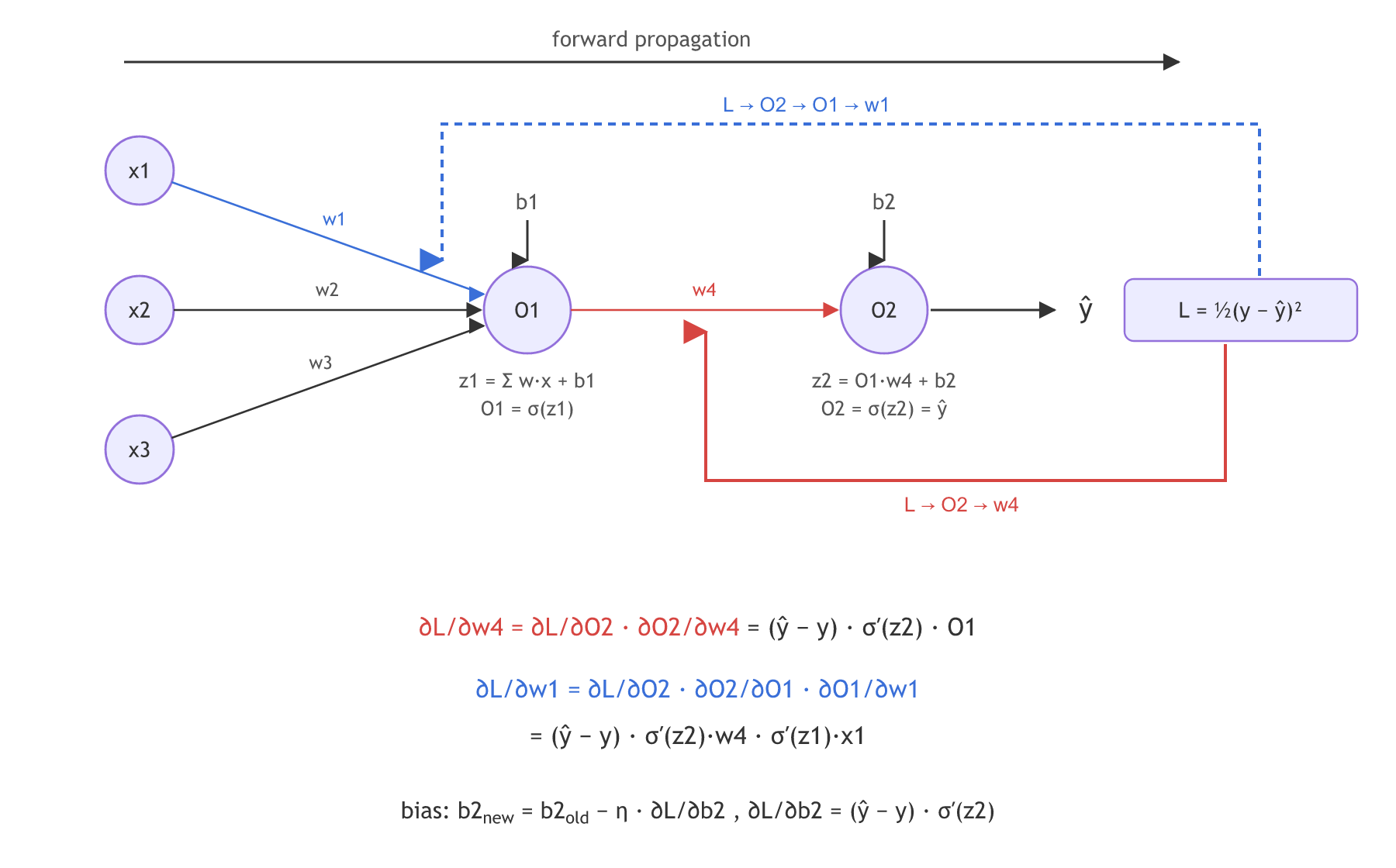
Name the outputs first. O1 is the hidden neuron's output: the inputs times their weights, plus the bias b1, then the activation. O2 is the output neuron's. The loss depends on O2, and O2 depends on w4. So the slope of the loss with respect to w4 is a chain of two derivatives:
The video "crosses" the two ∂O2 terms like fractions to show that the chain collapses back to ∂L/∂w4. Inside the output neuron there are two steps: z2 = O1·w4 + b2, then O2 = σ(z2). The board writes this as z = σ(O1·w4 + b), using z for the output; here z2 is the weighted sum before the sigmoid and O2 is the output after it.
A bias is updated with the same formula as a weight. For the output neuron's bias b2:
Finding the sigmoid derivative σ′ = σ(1 − σ)
Every factor that passes through a sigmoid neuron needs the derivative of σ. It has a short form in terms of σ itself:
The second fraction is 1 − σ(z), because 1 − 1/(1 + e^(−z)) = e^(−z)/(1 + e^(−z)). At z = 0, σ = 0.5 and σ′ = 0.5 × 0.5 = 0.25, its largest value; far from 0 it shrinks toward 0. That 0.25 ceiling is the heart of the Vanishing gradient problem lesson.
With it, each factor for w4 has a value. From L = ½(y − ŷ)², ∂L/∂O2 = ŷ − y. From z2 = O1·w4 + b2, ∂O2/∂w4 = σ′(z2)·O1, because the derivative of z2 with respect to w4 is O1. And ∂L/∂b2 is the same chain with 1 in place of O1.
Following the longer path to w1
w1 sits one layer further back. The loss depends on O2, O2 depends on O1, and O1 depends on w1, so the chain has three factors:
The middle factor is one hop back through the output neuron. O2 = σ(O1·w4 + b2), so ∂O2/∂O1 = σ′(z2)·w4. The last factor is the hidden neuron itself: O1 = σ(x1w1 + x2w2 + x3w3 + b1), so ∂O1/∂w1 = σ′(z1)·x1.
Right after this part the video splits ∂O2/∂O1 into ∂O2/∂w4 · ∂w4/∂O1. That split is wrong: w4 is a weight, not something computed from O1, so ∂w4/∂O1 has no meaning. The correct factor is σ′(z2)·w4, which is also how the notes write the hop ∂O31/∂O21 on their vanishing gradient page.
The video leaves w2 as an exercise. Its chain is w1's chain with a different last factor: ∂L/∂w2 = ∂L/∂O2 · ∂O2/∂O1 · ∂O1/∂w2, with ∂O1/∂w2 = σ′(z1)·x2. w3 works the same way with x3.
Adding the two paths through O21 and O22
The video's second network: x1 goes into one input neuron, then through w1 to the hidden neuron O11. O11 feeds two neurons in the next layer, O21 through w2 and O22 through w3. Both feed the output neuron O31, through w4 and w5, and O31 gives ŷ and the loss.
Now w1 reaches the loss along two routes: the top one through O21 and the bottom one through O22. Each route gives its own chain product, and the two products are added. The video compares it to an "or" between the routes: a change in w1 reaches the loss through either one, so both contributions count.
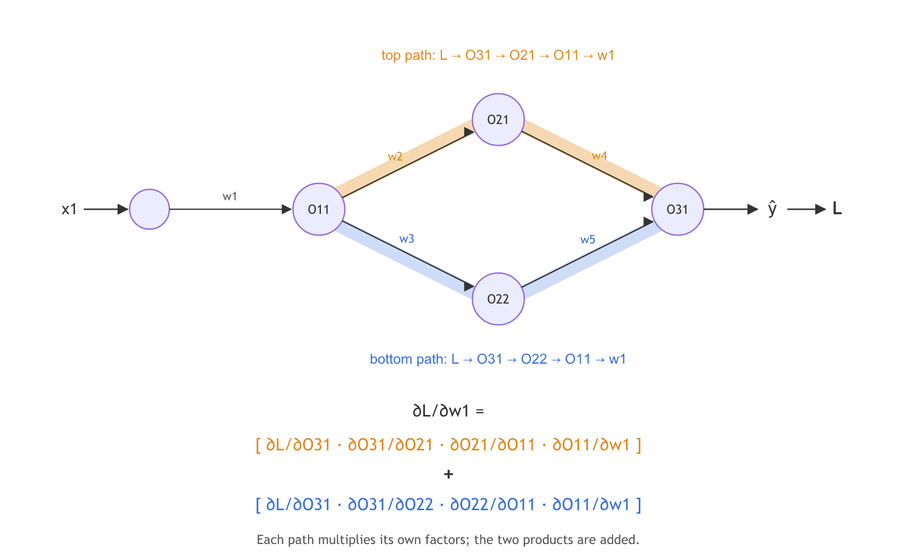
Both brackets start with ∂L/∂O31 and end with ∂O11/∂w1, so those two factors can be taken out once:
The notes' copy of this network writes O12 under the single neuron of the first hidden layer and uses ∂O22/∂O12 · ∂O12/∂w1 on the bottom path. That layer has one neuron, so both paths pass through O11, as on the video's board.
Computing the gradients of the 3-1-1 network
The run uses the forward pass from the backpropagation lesson (the sigmoid, x, y, weights and loss function) and works out every chain from the formulas above.
The local derivatives
A forward pass that keeps z1, O1, z2 and ŷ, then the three local derivatives every chain is built from:
z1 = x @ w + b1
O1 = sigmoid(z1)
z2 = O1 * w4 + b2
y_hat = sigmoid(z2)

dL_dO2 = y_hat - y                 # from L = 0.5 * (y - y_hat) ** 2
dO2_dz2 = y_hat * (1 - y_hat)      # sigmoid'(z2)
dO1_dz1 = O1 * (1 - O1)            # sigmoid'(z1)
Each weight's chain
Each gradient multiplies the factors on its path. The three input weights share one chain and differ only in their input, so one line computes all three:
grad_w4 = dL_dO2 * dO2_dz2 * O1
grad_b2 = dL_dO2 * dO2_dz2
dO2_dO1 = dO2_dz2 * w4             # sigmoid'(z2) * w4, one hop back
grad_w = dL_dO2 * dO2_dO1 * dO1_dz1 * x   # w1, w2, w3 together
grad_b1 = dL_dO2 * dO2_dO1 * dO1_dz1z1 = x @ w + b1
O1 = sigmoid(z1)
z2 = O1 * w4 + b2
y_hat = sigmoid(z2)
dL_dO2 = y_hat - y # from L = 0.5 * (y - y_hat) ** 2
dO2_dz2 = y_hat * (1 - y_hat) # sigmoid'(z2)
dO1_dz1 = O1 * (1 - O1) # sigmoid'(z1)
grad_w4 = dL_dO2 * dO2_dz2 * O1
grad_b2 = dL_dO2 * dO2_dz2
dO2_dO1 = dO2_dz2 * w4 # sigmoid'(z2) * w4, one hop back
grad_w = dL_dO2 * dO2_dO1 * dO1_dz1 * x # w1, w2, w3 together
grad_b1 = dL_dO2 * dO2_dO1 * dO1_dz1
print(f"z2: {z2:.5f} y_hat: {y_hat:.5f}")
print("sigmoid'(z2):", round(dO2_dz2, 5), " sigmoid'(z1):", round(dO1_dz1, 5))
print("dL/dw4:", round(grad_w4, 5), " dL/db2:", round(grad_b2, 5))
print("dL/dw1, dL/dw2, dL/dw3:", np.round(grad_w, 5))
print("dL/db1:", round(grad_b1, 6))
h = 1e-6
check = (loss(w, b1, w4 + h, b2) - loss(w, b1, w4 - h, b2)) / (2 * h)
print("nudging w4 gives:", round(check, 5))z2: 0.04519 y_hat: 0.51130 sigmoid'(z2): 0.24987 sigmoid'(z1): 0.18256 dL/dw4: -0.09277 dL/db2: -0.12211 dL/dw1, dL/dw2, dL/dw3: [-0.04236 -0.00178 -0.00178] dL/db1: -0.000446 nudging w4 gives: -0.09277
What the gradients show
- z2 = 0.04519 and ŷ = 0.51130: the forward pass at full precision. The notes round O1 to 0.759 first and get 0.04518 and 0.51129.
- σ′(z2) = 0.24987: z2 is close to 0, so the output neuron's derivative is almost the 0.25 maximum. σ′(z1) = 0.18256 is smaller because z1 = 1.151 is further from 0.
- dL/dw4 = −0.09277, the same number the nudge measured in the backpropagation lesson, and the last line confirms it.
- dL/dw1 = −0.04236 is 23.75 times dL/dw2: the two chains are identical except the last factor, x1 = 95 against x2 = 4, and 95 / 4 = 23.75.
- dL/db1 = −0.000446: the bias of the hidden neuron gets the smallest gradient. Its chain is w1's chain with 1 in place of the input, so it is dL/dw2 divided by 4, and that shared chain already passes w4 = 0.02 and two sigmoid derivatives.
Two paths in code
The same check on the two-path network. The video draws it without numbers, so the weights here are picked for the demo and the biases are left out:
x1, y = 1.0, 1.0
w1, w2, w3, w4, w5 = 0.5, -0.4, 0.8, 0.6, 0.3   # weights picked for the demo, no biases

def forward(w1):
    O11 = sigmoid(w1 * x1)
    O21, O22 = sigmoid(w2 * O11), sigmoid(w3 * O11)
    O31 = sigmoid(w4 * O21 + w5 * O22)
    return O11, O21, O22, O31

O11, O21, O22, O31 = forward(w1)
d = lambda o: o * (1 - o)          # sigmoid' written with the neuron's output
top = (O31 - y) * d(O31) * w4 * d(O21) * w2 * d(O11) * x1
bottom = (O31 - y) * d(O31) * w5 * d(O22) * w3 * d(O11) * x1
L = lambda w1: 0.5 * (y - forward(w1)[3]) ** 2
h = 1e-6
print("top path:", round(top, 6), "  bottom path:", round(bottom, 6))
print("sum:", round(top + bottom, 6), " nudging w1:", round((L(w1 + h) - L(w1 - h)) / (2 * h), 6))top path: 0.001286 bottom path: -0.001228 sum: 5.8e-05 nudging w1: 5.8e-05
The top path is positive and the bottom one negative: ŷ is below the label, so ∂L/∂O31 is negative, and the top path's w2 = −0.4 flips its sign once more. The two nearly cancel, and their sum, 0.000058, equals the slope measured by nudging w1. Either path alone would be wrong by a factor of more than 20.
Chain rule vs nudging each weight
| Chain rule (backward pass) | Nudging a weight | |
|---|---|---|
| What it gives | the exact slope | an estimate of the slope |
| Cost | one backward pass for all weights | two forward passes per weight |
| Used for | training | checking a hand-written backward pass |
| dL/dw4 in the run | −0.09277 | −0.09277 |
Where you use the chain rule
- Training any network: Keras and TensorFlow run the chain rule for you (automatic differentiation) on every batch; this lesson is what that machinery computes.
- Checking a hand-written backward pass: comparing the chain rule with a nudge, as the two runs did, is called gradient checking.
- Reading why gradients shrink: each hop multiplies by σ′(z)·w, which is where vanishing gradients come from.
Related
- Previous: Backpropagation and weight update
- Next: Vanishing gradient problem
- Print
grad_w * 0.01next tograd_w4 * 0.01: these are the changes one update with η = 0.01 makes. Which weight moves most? - In the two-path run, set
w3 = 0. What happens to the bottom path, and does the sum still match the nudge? - Change the label to
y = 0in the 3-1-1 run. Which gradients flip sign?
This is what real progress feels like.