Logistic regression
Logistic regression is a classification algorithm that passes a straight line θ₀ + θ₁x through the sigmoid function, so its output is a probability between 0 and 1 that a 0.5 threshold turns into a class.
Last updated: 05 Oct, 2026 · scikit-learn 1.9.1
The regression lessons predict a number. Many questions have a fixed set of answers instead: pass or fail, spam or not, cancer or not. Logistic regression is the first classification algorithm in the video, and it works very well for binary classification, two classes.
Predicting pass or fail with a straight line
The example: from a child's number of study hours (and play hours) predict whether the child passes or fails. There are two fixed categories, so this is binary classification. It can be extended to more classes, multiclass classification, but the video stays with two.
Keep one feature, the number of study hours. The board sketches the points without numbers; the table used here gives them hours: the students who studied 2, 3 and 4 hours failed, those who studied 5, 6 and 7 hours passed. Fail is written as 0 and pass as 1, and these are the training points.
Can linear regression solve it? It can draw a best fit line through the points, then use one rule: if hθ(x) is below 0.5 the output is 0, fail; if it is 0.5 or more the output is 1, pass. A new point predicted at 0.25 is a fail. A point far to the right lands above 0.5 on the extended line, a pass. So far it works.
Breaking the line with one outlier
Now add an outlier: a student who studied 12 hours and, of course, passed. The best fit line moves to reach it: it tilts and flattens. The point where it crosses 0.5 moves to the right, so a student who studied a little more than the old threshold is now predicted to fail, although by the old line the student passes. One outlier changed the answer for other students.
The second problem: the line gives values above 1 on the right and, projected back to the left, negative values. The answer can only be between 0 and 1. The fix for both is to squash the line, with the sigmoid function.
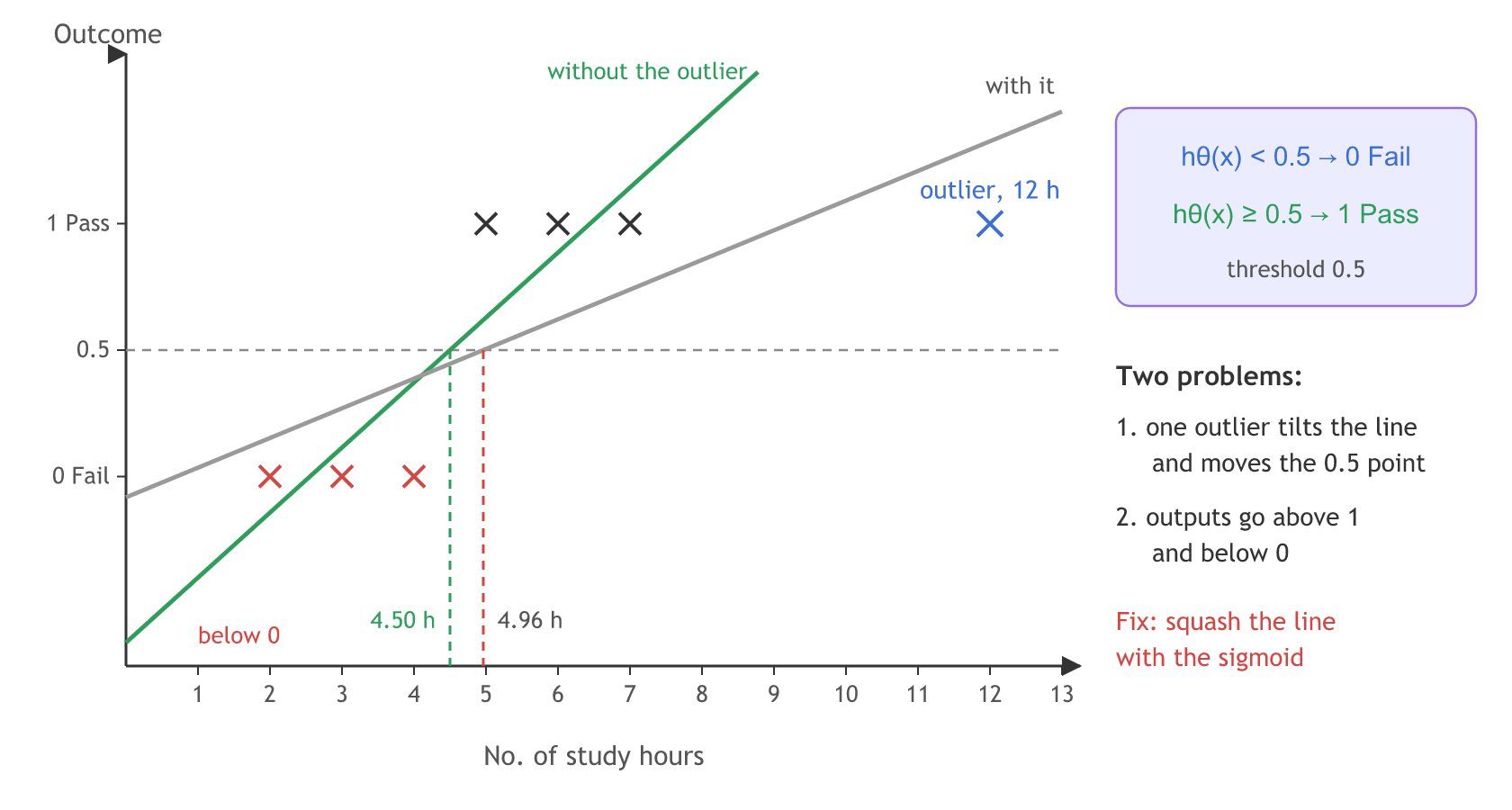
Fitted on these points, the line crosses 0.5 at exactly 4.5 hours, halfway between the last fail and the first pass. With the 12-hour student it crosses at 4.96 hours, so a student who studied 4.6 hours flips from pass to fail.
Squashing the line with the sigmoid
The hypothesis starts as a line: hθ(x) = θ₀ + θ₁x₁ + θ₂x₂ + … + θₙxₙ, written short as θᵀx. With one feature it is θ₀ + θ₁x. On top of this value logistic regression applies a function g that squashes it: hθ(x) = g(θ₀ + θ₁x). Let z = θ₀ + θ₁x. Then hθ(x) = g(z), with
This g is the sigmoid or logistic function. Its graph is an S: close to 0 on the far left, 1 on the far right, and exactly 0.5 at z = 0. Many texts write it σ(z) and call it the sigmoid activation; g and σ are the same function.
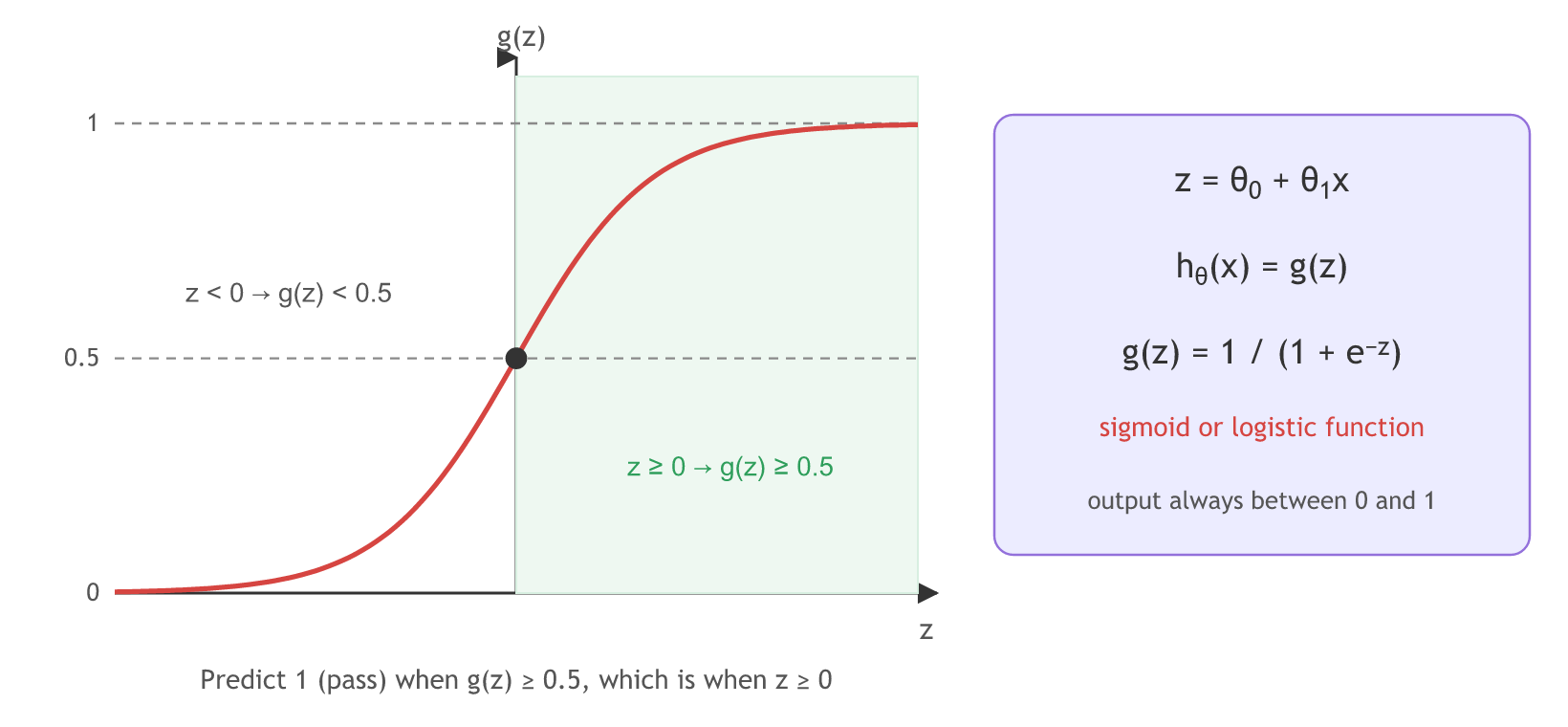
The key reading of the curve: g(z) ≥ 0.5 whenever z ≥ 0, and g(z) < 0.5 whenever z < 0. So the model predicts pass exactly when z = θ₀ + θ₁x is 0 or more. The line θ₀ + θ₁x = 0 is the decision boundary. The name comes from the two halves: regression builds the straight line, the logistic function squashes it. Does the squashing help with the outlier problem? The video says yes; the code checks it.
Fitting the study hours data
The LogisticRegression class
predict_proba returns the sigmoid output for each class, predict applies the 0.5 threshold. intercept_ is θ₀ and coef_ is θ₁, so the boundary z = 0 sits at x = −θ₀ / θ₁.
from sklearn.linear_model import LogisticRegression

model = LogisticRegression()
model.fit(hours, result)                 # hours: one column, result: 0 or 1
print(model.predict_proba([[4.6]]))      # [P(fail), P(pass)]
print(model.predict([[4.6]]))            # 1 when P(pass) >= 0.5
Linear and logistic with and without the outlier
import numpy as np
from sklearn.linear_model import LinearRegression, LogisticRegression

hours = np.array([2, 3, 4, 5, 6, 7]).reshape(-1, 1)
result = np.array([0, 0, 0, 1, 1, 1])                 # 0 = fail, 1 = pass
hours_out = np.vstack([hours, [[12]]])                       # the outlier: 12 hours, pass
result_out = np.append(result, 1)

for name, X, y in [("6 students", hours, result), ("with the 12 h outlier", hours_out, result_out)]:
    lin = LinearRegression().fit(X, y)
    cut = (0.5 - lin.intercept_) / lin.coef_[0]              # where the line crosses 0.5
    at_46 = lin.predict([[4.6]])[0]
    log = LogisticRegression().fit(X, y)
    boundary = -log.intercept_[0] / log.coef_[0, 0]          # where z = 0
    p_46 = log.predict_proba([[4.6]])[0, 1]
    print(f"{name}:")
    print(f"  linear:   0.5 at {cut:.2f} h, 4.6 h -> {at_46:.2f}")
    print(f"  logistic: boundary at {boundary:.2f} h, 4.6 h -> P(pass) {p_46:.2f}")

lin = LinearRegression().fit(hours, result)
print("linear output at 0 h and 10 h:", lin.predict([[0], [10]]).round(2))6 students: linear: 0.5 at 4.50 h, 4.6 h -> 0.53 logistic: boundary at 4.50 h, 4.6 h -> P(pass) 0.53 with the 12 h outlier: linear: 0.5 at 4.96 h, 4.6 h -> 0.46 logistic: boundary at 4.50 h, 4.6 h -> P(pass) 0.53 linear output at 0 h and 10 h: [-0.66 1.91]
Plotting the sigmoid
import numpy as np
import matplotlib.pyplot as plt

def g(z):
    return 1 / (1 + np.exp(-z))

for z in [-4, -1, 0, 1, 4]:
    print(f"g({z:2}) = {g(z):.3f}")

z = np.linspace(-6, 6, 200)
plt.plot(z, g(z), color="red")
plt.axhline(0.5, color="gray", linestyle="--")
plt.axvline(0, color="gray", linestyle="--")
plt.title("Sigmoid function")
plt.xlabel("z")
plt.ylabel("g(z)")
plt.show()g(-4) = 0.018 g(-1) = 0.269 g( 0) = 0.500 g( 1) = 0.731 g( 4) = 0.982
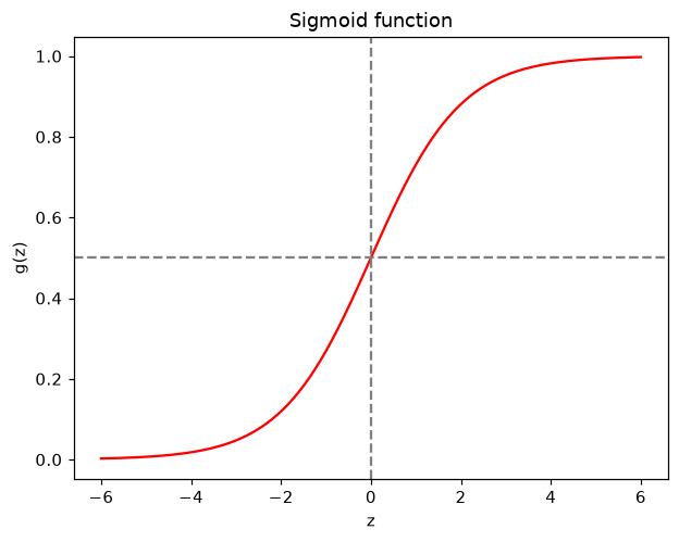
What the fits and the curve show
- The outlier moves the linear threshold. The 0.5 point slides from 4.50 to 4.96 hours, and the student at 4.6 hours drops from 0.53 (pass) to 0.46 (fail).
- The outlier does not move logistic regression. Its boundary stays at 4.50 hours and P(pass) at 4.6 hours stays 0.53. A point far on the correct side sits on the flat part of the S and barely pulls on the fit.
- The line leaves the 0 to 1 range. At 0 hours it predicts −0.66 and at 10 hours 1.91, neither of which is a valid answer.
- The sigmoid stays inside it. g(−4) = 0.018, g(0) = 0.5 and g(4) = 0.982: every output is a probability, and the 0.5 line meets the curve at z = 0.
Logistic regression vs linear regression
| Linear regression | Logistic regression | |
|---|---|---|
| Predicts | a number | a class, through a probability |
| Output range | any value, below 0 and above 1 | between 0 and 1 |
| Hypothesis | θ₀ + θ₁x | g(θ₀ + θ₁x), g = sigmoid |
| Decision | class 1 when g(z) ≥ 0.5, which is z ≥ 0 | |
| Effect of a far outlier | tilts the line and moves the threshold | almost none |
Where you use logistic regression
- Yes or no questions. Pass or fail, spam or not, a loan repaid or not, a tumour malignant or benign.
- When you need a probability. predict_proba gives a number you can rank or threshold, not only a label.
- As the first classifier to try. It is fast, and its coefficients show which way each feature pushes the answer.
predict returns classes 0 and 1, never the probability; ask predict_proba for that. And 0.5 is a choice, not a law: a cancer screen may flag a patient at a lower probability.Related
- Previous: Linear regression assumptions
- Next: Log loss
- Reference: scikit-learn: Logistic regression
- Move the outlier from 12 to 20 hours. The linear 0.5 point moves on to 5.28 hours, so now even a student at 5 hours, who passed, is predicted to fail; the logistic boundary stays at 4.50.
- Print
g(10)andg(-10): the sigmoid gets very close to 1 and 0 but never reaches them. - Fit LogisticRegression on the 6 students and print
predict_proba([[4.5]]). On the boundary the two probabilities are both about 0.5.
You understood something today that you didn't yesterday.