Naive Bayes
Naive Bayes is a classification algorithm that uses Bayes' theorem to pick the class with the highest probability for the features it is given.
Last updated: 04 Oct, 2026 · scikit-learn 1.9.1
Logistic regression learns a line that separates the classes. Naive Bayes takes a different route: it counts how often each feature value appears with each class, and turns those counts into probabilities with one formula, Bayes' theorem.
Telling independent and dependent events apart
The video starts with a die. Each face has a probability of 1/6: P(1) = 1/6, P(2) = 1/6, P(3) = 1/6. Getting a 1 on one roll does not change the chance of a 2 on the next roll. Events like these are independent events.
Then comes a bag of marbles: 3 red and 2 green, 5 in all. The first draw takes out a red marble, with probability 3/5. That red marble stays out. Now the bag holds 4 marbles, 2 of them green, so the chance of a green on the second draw is 2/4 = 1/2. The second draw depends on the first, because the bag got smaller. These are dependent events.
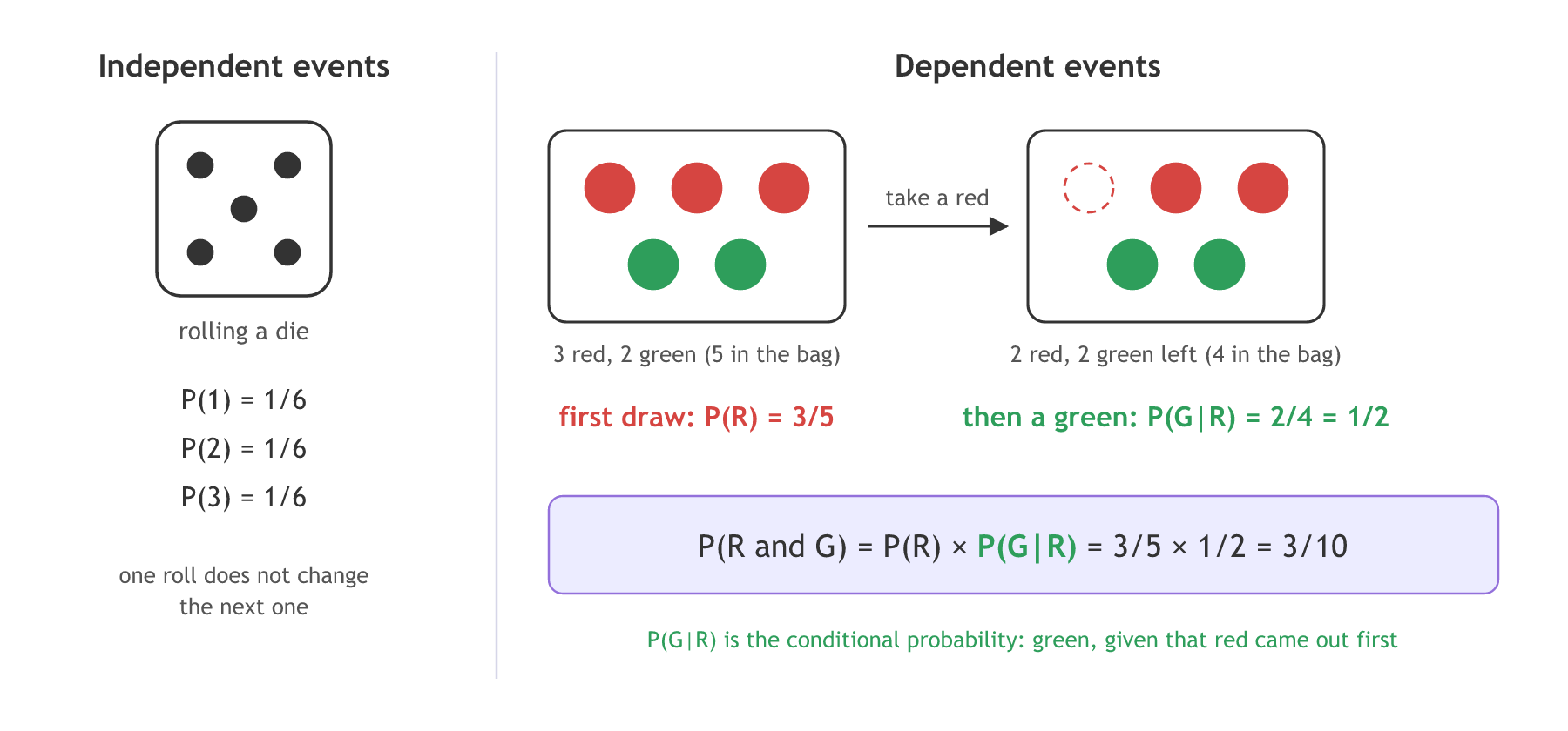
The chance of red first and then green multiplies the two steps. The second factor is written P(G | R), read "the probability of green given red". A probability that assumes another event has already happened is a conditional probability.
Deriving Bayes' theorem
The order of two events does not change the chance that both happen, so P(A and B) = P(B and A). The clip checks this on the marbles the other way round: green first has probability 2/5, then red given green is 3/4, and 2/5 × 3/4 = 3/10 again. Write each side with the conditional rule from the marbles:
Divide both sides by P(A) and you get Bayes' theorem. The board puts it in a box and calls it the crux of Naive Bayes: it turns a probability you can count, P(A | B), into the one you want, P(B | A).
Applying Bayes' theorem to features x1 to xn
A dataset has independent features x1, x2, ..., xn (the inputs) and an output y (the dependent feature). In Bayes' theorem, B becomes y and A becomes the whole row of features. The model is trained on rows where both are known, then asked about new rows where only the features are known.
The naive part is one assumption: once the class is known, the features do not depend on each other. Then the joint probability splits into one factor per feature, and every factor can be counted from the training table:
The board writes the factors as P(x1/y1), P(x2/y2) and so on; each factor is conditioned on the same class y, as written above. The output y can be binary (yes or no) or have more classes.
Scoring Yes and No for one record
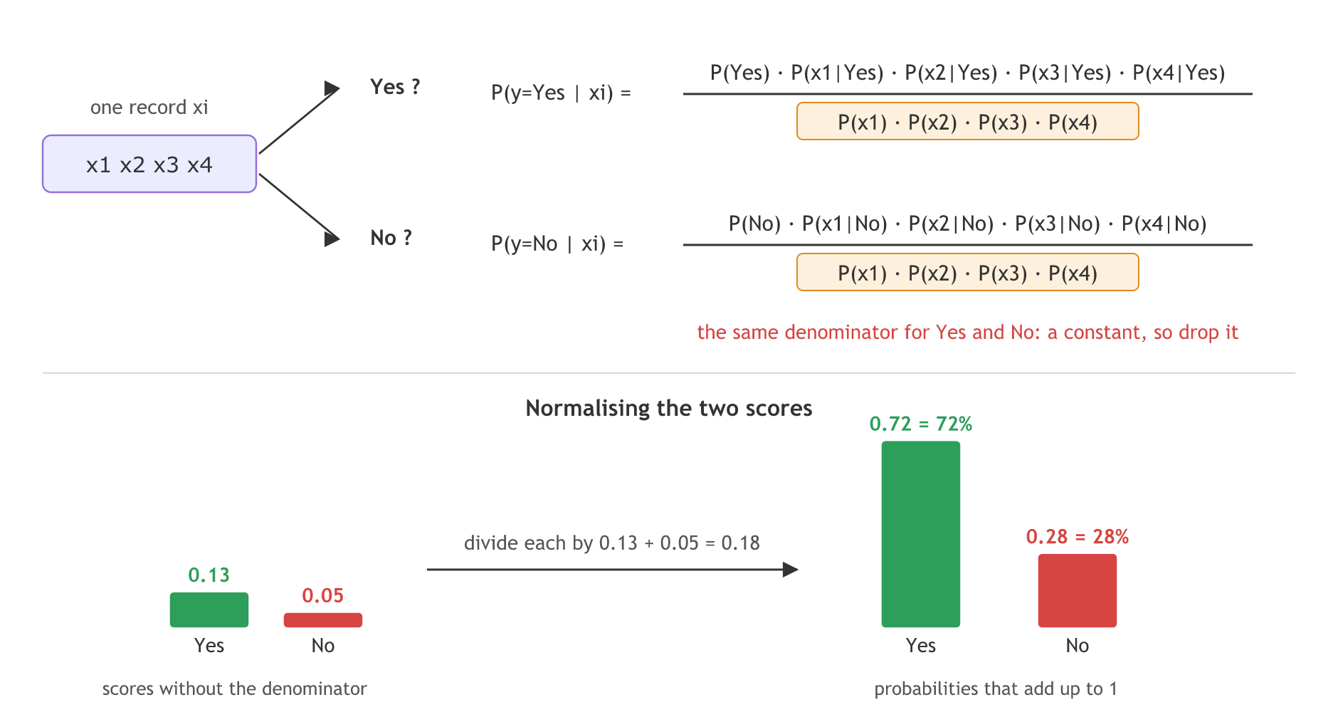
Take four features x1 to x4 and an output that is Yes or No. For a record xi you write the formula twice, once for each class:
Look at the two denominators: they are the same. For a given record the denominator is a constant, so it cannot change which class wins. Naive Bayes drops it and compares the two numerators.
Normalising the two scores
Without the denominator the two numbers are scores, not probabilities. Say a record scores 0.13 for Yes and 0.05 for No. Divide each by their sum to make them add up to 1:
The record gets the class with the larger share, Yes here.
Checking the marbles and Bayes' theorem in Python
Python's fractions module keeps 3/5 as 3/5 instead of 0.6, so the numbers match the board. Listing every ordered draw of two marbles checks the formulas by counting.
Listing every draw of two marbles
from fractions import Fraction
from itertools import permutations

bag = ["R", "R", "R", "G", "G"]          # 3 red, 2 green
draws = list(permutations(bag, 2))       # every ordered (first, second) pair
def prob(event):
    hits = sum(1 for d in draws if event(d))
    return Fraction(hits, len(draws))
Writing Bayes' theorem as a function
def bayes(p_b, p_a_given_b, p_a):
    # P(B | A) = P(B) * P(A | B) / P(A)
return p_b * p_a_given_b / p_ap_red_first = prob(lambda d: d[0] == "R")
after_red = list(bag)
after_red.remove("R") # the bag once a red marble is out
p_green_after_red = Fraction(after_red.count("G"), len(after_red))
p_red_then_green = prob(lambda d: d == ("R", "G"))
print("P(R) =", p_red_first)
print("P(R) x P(G|R) =", p_red_first * p_green_after_red)
print("counted P(R, G) =", p_red_then_green)
# Bayes: how likely was the first marble red, if the second one is green?
p_green_second = prob(lambda d: d[1] == "G")
print("P(G second) =", p_green_second)
print("Bayes P(R1|G2) =", bayes(p_red_first, p_green_after_red, p_green_second))
print("counted P(R1|G2)=", p_red_then_green / p_green_second)
# Normalising the two scores from the board
scores = {"Yes": 0.13, "No": 0.05}
total = sum(scores.values())
print({k: round(v / total, 2) for k, v in scores.items()})P(R) = 3/5
P(R) x P(G|R) = 3/10
counted P(R, G) = 3/10
P(G second) = 2/5
Bayes P(R1|G2) = 3/4
counted P(R1|G2)= 3/4
{'Yes': 0.72, 'No': 0.28}What the counts confirm
- P(R) = 3/5 and P(R) × P(G | R) = 3/10: the board's two steps. Counting all 20 ordered draws gives the same 3/10, so multiplying by the conditional probability is right.
- P(G second) = 2/5: before you look at the first marble, the second one is green 2 times in 5.
- Bayes gives 3/4, and so does counting: if the second marble is green, the first was red with probability 3/4. Bayes' theorem reversed the condition without listing any draws.
- 0.72 and 0.28: the board's scores 0.13 and 0.05 become probabilities once each is divided by their sum.
Naive Bayes vs logistic regression
| Naive Bayes | Logistic regression | |
|---|---|---|
| What it learns | Counts: P(class) and P(feature value | class) | Weights of a line, by gradient descent |
| Training | One pass of counting, very fast | Many steps of optimisation |
| Key assumption | Features independent given the class | Log-odds are a linear function of the features |
| Probabilities | Often too extreme, because of the assumption | Usually well calibrated |
| Small data | Works with few rows | Needs more rows to fit the weights |
Where you use Naive Bayes
- Spam filtering: each word in an email is a feature, and P(word | spam) is counted from labelled emails.
- Text classification: sorting news articles by topic or reviews by sentiment, where there are thousands of word features.
- A fast first baseline: it trains in one pass, so it gives a score to beat before you try slower models.
Related
- Previous: One-vs-rest logistic regression
- Next: Naive Bayes worked example
- Reference: scikit-learn user guide, Naive Bayes
- Change the bag to 4 red and 1 green marble. Before you run it, work out P(R) × P(G | R) by hand (4/5 × 1/4), then check the printed value.
- Change the scores to {"Yes": 0.02, "No": 0.06}. Which class wins, and with what share?
- Use
probto count P(G first and G second). Is it 2/5 × 1/4?
Slow is fine. Stopping is the only problem.