
Retraining strategies
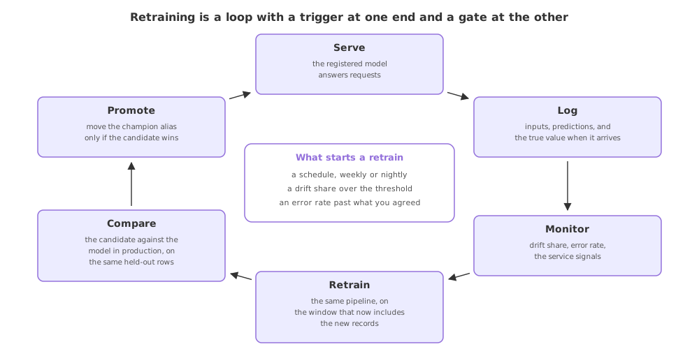
Retraining is fitting the model again on a window of data that now includes the records it was getting wrong. The strategies differ in one thing: what starts it. A clock, a monitoring threshold, or every record as it arrives.
Last updated: 19 Oct, 2026 · MLOps
The signals to monitor ends with a number over a threshold. This lesson is what happens next, and the video the course takes it from is clear that there is no single approach: a model is retrained on a schedule, on a trigger, or one observation at a time, and the choice follows how fast the data moves and how expensive a fit is.
Choosing what starts the retrain
| Strategy | What starts it | Costs | Fits when |
|---|---|---|---|
| Scheduled | A clock: nightly, weekly, monthly | A full fit every run, most of them unnecessary | The data moves steadily and a fit is cheap |
| Triggered | A drift share or an error rate over its threshold | Monitoring has to be trustworthy before it can hold the trigger | Fits are expensive or the data moves in jumps |
| Incremental | Every new record, as it arrives | A model and a library that support partial fitting | Live streams, where refitting from scratch is out of reach |
| Manual | A person, after reading the dashboard | Somebody has to remember | Early on, while you learn what normal looks like |
Scheduled and triggered are not rivals. The common production shape is a weekly schedule with a drift check at the front of it: the clock wakes the pipeline up, the check decides whether a fit is worth the compute, and a human is paged only when the fit does not help.
The clip's loop keeps the model learning from each new chunk as it arrives; this course retrains in full on a schedule through the DVC pipeline, because the student-performance model is small enough to refit from scratch.
Training once against training continuously
The video draws the difference as two pictures. In the first, a model is fitted offline on a dataset, scored, deployed, and left alone; every retrain starts from zero. In the second, live data is collected from a stream into storage and taken in chunks, and the model is updated one observation at a time, without being fitted from scratch. That second shape is incremental, also called online learning, and its appeal is that a model can keep up with data far larger than memory and can absorb a category it has never seen without a full refit.
It also costs something. An incrementally updated model has no clean held-out set to score against, it can be dragged off course by a bad batch, and most of the tooling in this course, a versioned dataset and a registered artifact per run, assumes a fit with a beginning and an end. A full refit on a window stays the default for tabular models of this size, and the course's running example uses it.
Picking the window to fit on
- Everything, forever. Simple, and it dilutes the new records: 358 recent rows against years of history barely move the fit.
- A rolling window. The last n months only, so the model is meant to forget old behaviour. The risk is losing a seasonal pattern that only appears once a year.
- Everything, with the recent rows weighted. Keeps history and still leans towards what is happening now; sample weights are the usual way.
- Whatever you choose, version it. The window is part of the model, so the data version that produced a run belongs next to its metrics, which is what the DVC part of the course set up.
Building the window the retrain is fitted on
Six in ten of the 358 new students, 214 of them, go into the retraining window. The other 144 are held back, so there are records neither model has been fitted on, which is the only fair way to compare them. fit_forest is the wrapper from Why a live model decays: the course's preprocessor and forest, fitted on whatever frame it is handed.
# 60% of the new records join the window, 40% are kept back to judge with
new_records, held_back = train_test_split(cur, test_size=0.4, random_state=42)
window = pd.concat([ref, new_records])
Comparing the stale model with the candidate
Two fits of the same function on two windows, scored on the same held-back rows. This is the comparison the gate in front of a promotion makes, and it is the only evidence that a retrain was worth running.
from sklearn.metrics import mean_absolute_error, r2_score

stale = fit_forest(ref)         # what production is still serving
candidate = fit_forest(window)  # the same pipeline, the wider window

# both are judged on records neither of them was fitted on
truth = held_back.math_score
features = held_back.drop(columns=["math_score"])
for name, model in [("stale", stale), ("candidate", candidate)]:
    pred = model.predict(features)
print(f"{name:10} r2 {r2_score(truth, pred):.4f} MAE {mean_absolute_error(truth, pred):.4f}")stale r2 0.7629 MAE 5.4628 candidate r2 0.8116 MAE 4.7176
What the comparison earned
- The candidate wins on both measures. Adding 214 records of the new population to a window of 642 lifted r2 and took about three quarters of a mark off the average error.
- The gain came from the new records, not from more data. They are the only rows that carry the population the held-back students belong to, which is why a retrain on a drifted window is worth running at all.
- A retrain that does not win is a retrain you throw away. The comparison is the gate: if the candidate had lost, the correct action is to leave production alone and go and look at why.
- Both numbers come from the same held-back rows. Scoring two models on two different test sets proves nothing, and it is the easiest mistake to make in a retraining pipeline.
Related
- Previous: The signals to monitor
- Next: Orchestrating with Airflow
- See also: The model registry
- Change test_size to 0.8 so only 71 new records join the window, and see how much of the gain survives.
- Fit the candidate on new_records alone instead of the combined window, and watch what dropping the history costs.
- Print both models' scores on the reference students as well, and check that the candidate did not buy its gain by forgetting them.
You understood something today that you didn't yesterday.