
LoRA and QLoRA
LoRA (low-rank adaptation) is a parameter-efficient fine-tuning method that freezes a model's weights and trains two small matrices, B and A, whose product is added to each chosen weight matrix; QLoRA is LoRA run on a base model stored in 4-bit.
Last updated: 08 Oct, 2026 · NumPy
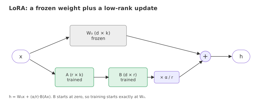
Full fine-tuning updates every weight, and the memory for that is out of reach on one GPU (see Fine-tuning LLMs). LoRA (Hu et al., 2021) changes what is trained: the pre-trained matrix W0 stays as it is, and the change to it is learned as a product of two thin matrices.
Writing the weight update as B times A
The paper's equation says that the new weight is the pre-trained weight plus B multiplied by A. For a weight matrix W0 with d rows and k columns, B has d rows and r columns, A has r rows and k columns, and r, the rank, is a small number chosen before training. LoRA never builds a full-size change matrix. B and A are created and trained directly, with the product BA standing in for the change.
Starting B at zero
A starts as small random numbers and B starts as zeros, so BA is zero at the first step and the model begins exactly where the pre-trained model was.
W0 = rng.normal(size=(d, k))               # frozen pretrained weight
A = rng.normal(0, 0.1, size=(r, k))        # r x k, small random start
B = np.zeros((d, r))                       # d x r, zeros: BA starts at 0
The forward pass and the merge
h = W0 @ x + (alpha / r) * (B @ (A @ x))      # frozen path plus the low-rank path
W_merged = W0 + (alpha / r) * (B @ A) # one matrix with the update folded inimport numpy as np
rng = np.random.default_rng(0)
d, k, r, alpha = 8, 8, 2, 4
W0 = rng.normal(size=(d, k)) # frozen pretrained weight
A = rng.normal(0, 0.1, size=(r, k)) # r x k, small random start
B = np.zeros((d, r)) # d x r, zeros: BA starts at 0
x = rng.normal(size=k)
h = W0 @ x + (alpha / r) * (B @ (A @ x)) # LoRA forward pass
print("before training, h equals W0 @ x:", np.allclose(h, W0 @ x))
B = rng.normal(0, 0.1, size=(d, r)) # pretend training has moved B
h = W0 @ x + (alpha / r) * (B @ (A @ x))
W_merged = W0 + (alpha / r) * (B @ A) # merge once, then serve W_merged
print("merged weight gives the same h:", np.allclose(h, W_merged @ x))
print("trainable:", A.size + B.size, "of", W0.size, "in this one matrix")before training, h equals W0 @ x: True merged weight gives the same h: True trainable: 32 of 64 in this one matrix
Reading the zero start and the merge
- At the start h equals W0 @ x (True): with B at zero the adapter adds nothing.
- The merged weight W0 + (alpha/r)BA gives the same h (True) after B has moved. After training, the update is folded into one matrix of the original shape, so a merged model runs at the speed of the base model.
- This 8 x 8 matrix has 32 trainable values out of 64 at r = 2. Savings need a large matrix and a small rank, as the next block shows.
Counting the parameters of a LoRA update
B holds d × r values and A holds r × k, so the update has r × (d + k) trainable values against d × k for the full matrix. It is smaller only while r is below d·k / (d + k).
d = k = 4096                                          # one attention projection of a 7B model
print("full matrix:", d * k)
for r in (1, 8, 64):
    n = r * (d + k)                                   # B is d x r, A is r x k
    print(f"r = {r:2}: B and A hold {n:>7,} values = {n / (d * k):.2%} of the matrix")
print("break-even rank for 3 x 3:", 3 * 3 / (3 + 3))
print("3 x 3 with r = 1 holds", 1 * (3 + 3), "values; with r = 2 it holds", 2 * (3 + 3))full matrix: 16777216 r = 1: B and A hold 8,192 values = 0.05% of the matrix r = 8: B and A hold 65,536 values = 0.39% of the matrix r = 64: B and A hold 524,288 values = 3.12% of the matrix break-even rank for 3 x 3: 1.5 3 x 3 with r = 1 holds 6 values; with r = 2 it holds 12
For a 4096 x 4096 projection, r = 8 means 65,536 values, 0.39% of the 16,777,216 in the matrix; r = 1 is 0.05% and r = 64 is 3.12%. A 3 x 3 matrix breaks even at r = 1.5: with r = 1 the factors hold 6 values for the 9 of the matrix, and with r = 2 they hold 12, which is more.
Counting the trainable parameters of GPT-3 with LoRA
The paper adapts the query and value matrices in each of the 96 layers of GPT-3 175B, whose model dimension is 12,288. Each adapted matrix has 2 × 12,288 × r values.
layers, d = 96, 12288                                 # GPT-3 175B
for r in (1, 2, 4, 8, 64):
    n = layers * 2 * r * (d + d)                      # W_q and W_v in every layer
print(f"r = {r:2}: {n:>11,} trainable = {n / 1e6:.1f}M")r = 1: 4,718,592 trainable = 4.7M r = 2: 9,437,184 trainable = 9.4M r = 4: 18,874,368 trainable = 18.9M r = 8: 37,748,736 trainable = 37.7M r = 64: 301,989,888 trainable = 302.0M
The paper's GPT-3 results list LoRA with 4.7M and 37.7M trainable parameters, which are the r = 1 and r = 8 rows of the block; the other ranks are computed here. Against the 175 billion weights, that is the reduction of about 10,000 times the paper cites in its abstract. For r = 4 on W_q and W_v the paper reports the checkpoint falling from 350 GB to 35 MB.
Choosing the rank, alpha and layers
- Rank r is a hyperparameter you set; nothing computes it. The paper finds ranks of 1 to 8 enough for its tasks on W_q and W_v, and 8 is a common default. A higher rank gives the update more freedom, which helps when the behaviour to learn is far from what the base model does.
- Alpha scales the update by alpha / r. Keeping alpha fixed while r changes keeps the size of the update comparable between ranks.
- The paper adapts W_q and W_v. The QLoRA paper adapts every linear layer, which is what
target_modules="all-linear"does in the peft library. The next block counts both for Llama 2 7B.
layers, d, ffn, vocab = 32, 4096, 11008, 32000        # Llama-2 7B config
attn = 4 * d * d                                      # q, k, v, o projections
mlp = 3 * d * ffn                                     # gate, up, down
total = layers * (attn + mlp + 2 * d) + 2 * vocab * d + d
print("model parameters:", f"{total:,}")
for name, per_layer in [("q_proj and v_proj", 2 * (d + d)),
                        ("all linear layers", 4 * (d + d) + 3 * (d + ffn))]:
    for r in (8, 64):
        n = layers * per_layer * r
print(f"{name:18} r = {r:2}: {n:>12,} trainable = {n / total:.2%}")model parameters: 6,738,415,616 q_proj and v_proj r = 8: 4,194,304 trainable = 0.06% q_proj and v_proj r = 64: 33,554,432 trainable = 0.50% all linear layers r = 8: 19,988,480 trainable = 0.30% all linear layers r = 64: 159,907,840 trainable = 2.37%
Llama 2 7B has 6,738,415,616 parameters. On q_proj and v_proj, r = 8 trains 4,194,304 values (0.06%) and r = 64 trains 33,554,432 (0.50%). On all linear layers, r = 8 trains 19,988,480 (0.30%) and r = 64 trains 159,907,840 (2.37%).
QLoRA: LoRA on a 4-bit base
QLoRA (Dettmers et al., 2023) is LoRA on top of a quantized base. The pre-trained weights are stored in 4-bit and frozen. During the forward and backward pass each block of them is dequantized to a 16-bit compute type for the matrix multiply, and only the LoRA matrices, kept in 16-bit, receive gradients. The adapters are the same B and A as in LoRA. The clip ends on the bitsandbytes configuration (load in 4-bit, the nf4 type, a 16-bit compute dtype) and a LoRA configuration with rank 8, target modules and the causal language modelling task type.
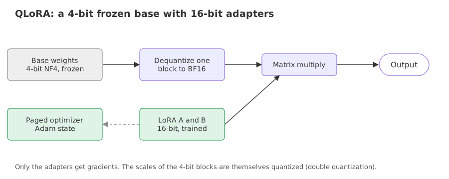
The paper reports that these pieces take a 65-billion-parameter model from more than 780 GB of GPU memory for 16-bit fine-tuning to under 48 GB, one GPU. Three ideas make it work: the NF4 data type, double quantization and paged optimizers.
The two configurations
import torch
from transformers import BitsAndBytesConfig

bnb = BitsAndBytesConfig(
    load_in_4bit=True,                      # store the base in 4-bit
    bnb_4bit_quant_type="nf4",               # the NF4 data type
    bnb_4bit_compute_dtype=torch.bfloat16,  # dequantize to bf16 for the matmul
    bnb_4bit_use_double_quant=True,         # quantize the scales too
)from peft import LoraConfig
lora = LoraConfig(r=8, lora_alpha=16, lora_dropout=0.05,
target_modules="all-linear", task_type="CAUSAL_LM")NF4: levels placed where the weights are
Pre-trained weights are roughly bell-shaped, with most values near zero. Evenly spaced 4-bit levels waste codes on the thin tails. NF4 (normal float 4) places its 16 levels at the quantiles of a normal distribution, so each level serves the same share of weights. The block builds a quantile-based 16-level grid and compares it with an even grid on 100,000 normal values, one scale for the whole array. The published NF4 table differs in detail: it is built so that zero is represented exactly, and the scale is set per block of weights.
import numpy as np
from statistics import NormalDist

rng = np.random.default_rng(42)
w = rng.normal(0, 1, 100_000)                         # weights are roughly bell shaped

nd = NormalDist()
p = (np.arange(16) + 0.5) / 16                        # 16 equal-probability slices
levels = np.array([nd.inv_cdf(v) for v in p])
levels /= np.abs(levels).max()                        # normalised to [-1, 1]

def snap(v, grid):
    scale = np.abs(v).max()
    g = grid * scale
    return g[np.abs(v[:, None] - g[None, :]).argmin(axis=1)]

uniform = np.linspace(-1, 1, 16)
for name, grid in [("uniform 4-bit", uniform), ("normal-quantile 4-bit", levels)]:
    err = np.abs(snap(w, grid) - w).mean()
print(f"{name:22} mean error {err:.4f}")uniform 4-bit mean error 0.1669 normal-quantile 4-bit mean error 0.1140
The mean error is 0.1669 with evenly spaced levels and 0.1140 with the quantile-based levels, the same 16 codes placed better.
Double quantization and paged optimizers
Block-wise quantization stores one scale per block, a 32-bit float for every 64 weights, which costs 0.5 bits per weight. Double quantization quantizes those scales to 8 bits in groups of 256. Paged optimizers keep Adam's state in memory that can move to CPU RAM when the GPU runs out during a spike, so a long sequence does not end the run.
block, const_bits, const_block = 64, 32, 256
plain = const_bits / block                            # one FP32 scale per 64 weights
double = 8 / block + const_bits / (block * const_block)   # scales stored in 8 bits, with their own scale
print(f"extra bits per weight, plain  : {plain:.4f}")
print(f"extra bits per weight, double : {double:.4f}")
print(f"saved: {plain - double:.3f} bits per weight")
n = 6_476_005_376                                     # Llama-2 7B linear-layer weights
for name, extra in [("4-bit + FP32 scales", plain), ("4-bit + double quantization", double)]:
print(f"{name:28} {n * (4 + extra) / 8 / 1e9:.2f} GB")extra bits per weight, plain : 0.5000 extra bits per weight, double : 0.1270 saved: 0.373 bits per weight 4-bit + FP32 scales 3.64 GB 4-bit + double quantization 3.34 GB
The scales cost 0.5000 bits per weight plain and 0.1270 with double quantization, a saving of 0.373 bits per weight. On the 6,476,005,376 linear-layer weights of Llama 2 7B that is 3.64 GB against 3.34 GB.
LoRA vs QLoRA vs full fine-tuning
| Full fine-tuning | LoRA | QLoRA | |
|---|---|---|---|
| Base weights | Trained | Frozen, 16-bit | Frozen, 4-bit NF4 |
| Trained values | All of them | B and A only | B and A only |
| Memory for a 7B model | 107.8 GB with FP32 Adam | 14.0 GB | 4.4 GB |
| After training | One model | Adapter, or merge it into the base | Adapter; reload the base in 16-bit to merge |
| Quality | The reference | Close to full fine-tuning in the paper's tests | Matches 16-bit fine-tuning in the paper's tests |
Where you use LoRA and QLoRA
- One base model, many tasks. Each task is a small adapter file; the base is stored once.
- Fine-tuning on one GPU. QLoRA is how a 7B model is tuned on a free Colab T4; see Fine-tuning Llama with QLoRA.
- Serving. Merge an adapter into the base for no extra latency, or load adapters on demand.
Related
- Previous: Fine-tuning LLMs
- Next: Fine-tuning Llama with QLoRA
- See also: Quantization
- In the LoRA layer block, set r to 4 and read how the trainable count changes against the 64 values of the matrix.
- In the 4096 x 4096 block, add r = 16 and r = 32 to the loop.
- In the NF4 block, change the weights to a uniform distribution with rng.uniform(-1, 1, 100_000) and compare the two errors.
You understood something today that you didn't yesterday.