Activation functions
An activation function is a function applied to a neuron's weighted sum z that sets the neuron's output and adds the non-linearity a network needs to learn curved patterns.
Last updated: 05 Oct, 2026 · NumPy
The Vanishing gradient problem lesson ended with the video's fix: use another activation function. This lesson covers why a neuron needs one at all, then the first two the video compares, sigmoid and tanh, each with its derivative, the part backpropagation uses.
Seeing why a network needs an activation
Without an activation, every layer computes z = Wx + b, a linear function. A linear function of a linear function is still linear, so a stack of such layers equals one layer, however deep it is. The run builds two layers with no activation between them and the single layer they collapse into:
import numpy as np
rng = np.random.default_rng(0)

x = rng.normal(0, 1, 3)                       # one record, 3 inputs
W1, b1 = rng.normal(0, 1, (4, 3)), rng.normal(0, 1, 4)
W2, b2 = rng.normal(0, 1, (1, 4)), rng.normal(0, 1, 1)

two_layers = W2 @ (W1 @ x + b1) + b2          # no activation in between
W, b = W2 @ W1, W2 @ b1 + b2                  # one layer with merged weights
print("two linear layers:", np.round(two_layers, 6))
print("one linear layer: ", np.round(W @ x + b, 6))two linear layers: [-0.028818] one linear layer: [-0.028818]
Both lines print the same numbers. With a non-linear activation between the layers that merge is impossible, which is what lets a network bend its decision boundary; this is the "solve non-linear problems" point the video makes for the sigmoid in each neuron.
Plotting the sigmoid and its derivative
The video's notebook shows each activation as two plots: on the left the function, used in the forward pass, and on the right its derivative, used in backpropagation. For sigmoid:
import numpy as np
import matplotlib.pyplot as plt

z = np.linspace(-10, 10, 401)
s = 1 / (1 + np.exp(-z))                      # sigmoid
ds = s * (1 - s)                              # its derivative

fig, (a, b) = plt.subplots(1, 2, figsize=(9, 3.4))
a.plot(z, s)
a.axhline(0.5, ls="--", c="grey")
a.set_title("sigmoid σ(z)")
a.set_xlabel("z")
b.plot(z, ds, c="tab:orange")
b.set_title("derivative σ′(z)")
b.set_xlabel("z")
plt.tight_layout()
plt.show()
print("σ(0) =", s[200], "  largest σ′ =", ds.max(), "at z =", z[ds.argmax()])
print("σ′ at z = 5:", round(ds[300], 4), " at z = 10:", round(ds[400], 6))σ(0) = 0.5 largest σ′ = 0.25 at z = 0.0 σ′ at z = 5: 0.0066 at z = 10: 4.5e-05
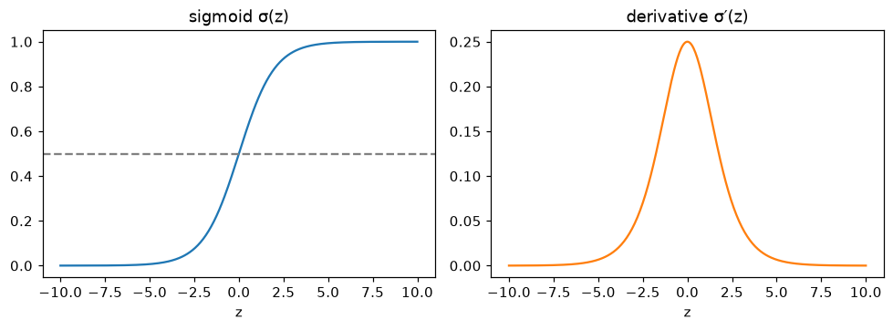
- σ(0) = 0.5 and the largest σ′ is 0.25 at z = 0, the ceiling behind the vanishing gradient.
- σ′ is 0.0066 at z = 5 and 0.000045 at z = 10: once the input is a little away from the origin, the gradient is almost 0. A neuron there barely learns.
The notebook's list for sigmoid: its advantages are a smooth gradient, an output between 0 and 1 for every neuron, and clear predictions close to 1 or 0. Its three disadvantages are that it is prone to vanishing gradients, its output is not zero centred, and the exponential is slow to compute (the 1/(1 + e^(−z)) formula takes more time than a comparison or a multiplication).
Understanding zero-centred outputs
The video draws a curve that passes through the origin, with negative values on one side and positive on the other: a zero-centred curve. Sigmoid never goes below 0, so it is not zero centred. The video's point is that a zero-centred curve makes the weight update more efficient. The notes draw the same idea with data: a cloud of points far from the origin, moved onto it by standardization.
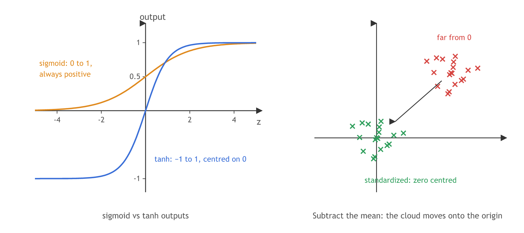
Here is why. A neuron's weight gradient is ∂L/∂wᵢ = δ · xᵢ, where δ = ∂L/∂z is one number for the whole neuron and xᵢ are its inputs, the previous layer's outputs. If every input is positive, as sigmoid outputs are, every weight gradient of that neuron has the sign of δ:
import numpy as np

delta = -0.3                                  # dL/dz of one neuron in the next layer
inputs_sigmoid = np.array([0.2, 0.7, 0.9])    # sigmoid outputs: all positive
inputs_tanh = np.array([-0.6, 0.4, 0.7])      # tanh outputs: both signs
print("weight gradients, sigmoid inputs:", delta * inputs_sigmoid)
print("weight gradients, tanh inputs: ", delta * inputs_tanh)weight gradients, sigmoid inputs: [-0.06 -0.21 -0.27] weight gradients, tanh inputs: [ 0.18 -0.12 -0.21]
With sigmoid inputs all three gradients are negative, so all three weights must rise together on this step and fall together on another. Reaching a point where one weight should go up and another down then takes a zig-zag of steps. With zero-centred inputs the signs can differ, so each weight moves its own way.
Comparing tanh with sigmoid
The second activation is tanh, the hyperbolic tangent. Its output runs from −1 to 1 and its derivative from 0 to 1, against 0 to 0.25 for sigmoid:
The video's question: does tanh prevent the vanishing gradient problem? Not in a very deep network. Its derivative is 1 only at z = 0 and falls toward 0 in both tails, so a long chain of tanh derivatives can still be tiny. What tanh does fix is the centring: it passes through the origin, so it is zero centred. In a binary classification problem the notebook's advice is tanh in the hidden layers and sigmoid in the output layer.
Reading the notebook aloud, the video says the two curves are "relatively smaller" and that a small gradient "is conducive to weight update". The notebook says the curves are relatively similar, and that a small gradient for large or small inputs is not conducive to weight updates.
import numpy as np
import matplotlib.pyplot as plt

z = np.linspace(-10, 10, 401)
t = np.tanh(z)
dt = 1 - t ** 2                               # tanh derivative
s = 1 / (1 + np.exp(-z))
ds = s * (1 - s)                              # sigmoid derivative

fig, (a, b) = plt.subplots(1, 2, figsize=(9, 3.4))
a.plot(z, t)
a.set_title("tanh(z)")
a.set_xlabel("z")
b.plot(z, dt, label="tanh′(z)")
b.plot(z, ds, label="σ′(z)", c="tab:orange")
b.set_title("derivatives")
b.set_xlabel("z")
b.legend()
plt.tight_layout()
plt.show()
for zv in [0, 1, 2, 4]:
    i = 200 + zv * 20
print(f"z = {zv}: tanh′ = {dt[i]:.4f} σ′ = {ds[i]:.4f}")z = 0: tanh′ = 1.0000 σ′ = 0.2500 z = 1: tanh′ = 0.4200 σ′ = 0.1966 z = 2: tanh′ = 0.0707 σ′ = 0.1050 z = 4: tanh′ = 0.0013 σ′ = 0.0177
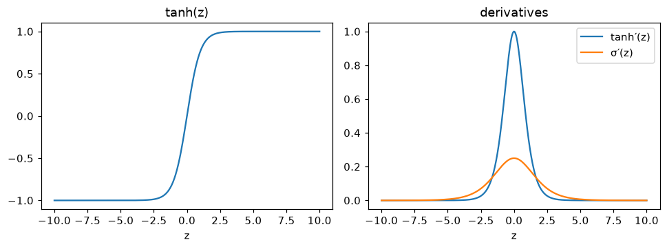
What the two derivatives show
- At z = 0, tanh′ is 1 and σ′ is 0.25: four times more gradient passes through a tanh neuron near the origin.
- At z = 2, tanh′ is 0.0707 and σ′ is 0.105: tanh's derivative falls faster, and away from the origin it is not the larger one.
- At z = 4 both are close to 0 (0.0013 and 0.0177): saturated neurons pass almost no gradient with either function, so deep tanh networks can still vanish.
Sigmoid vs tanh
| Sigmoid | tanh | |
|---|---|---|
| Formula | 1 / (1 + e^(−z)) | (e^z − e^(−z)) / (e^z + e^(−z)) |
| Output range | 0 to 1 | −1 to 1 |
| Zero centred | no | yes |
| Derivative range | 0 to 0.25 | 0 to 1 |
| Vanishing gradient | yes | yes, in very deep networks |
| Cost | one exponential | exponentials (slower) |
| Typical place | output layer, binary classification | hidden layers of small networks |
Where you use sigmoid and tanh
- Binary classification output: one sigmoid neuron gives a value between 0 and 1, and 0.5 is the usual threshold; in Keras,
Dense(1, activation="sigmoid"). - Small networks: tanh in the hidden layers of a shallow network trains better than sigmoid because its outputs are zero centred.
- Gates inside recurrent cells: LSTM and GRU cells use sigmoid to squash a gate into 0 to 1 and tanh for the values that pass through it.
Related
- Previous: Vanishing gradient problem
- Next: ReLU and its variants
- In the sigmoid run, print
ds[220], the derivative at z = 1. Is it closer to 0.25 or to 0? - Check that tanh is a stretched sigmoid: compare
np.tanh(1.0)with2 / (1 + np.exp(-2.0)) - 1. - In the two-layer run, put
np.tanharoundW1 @ x + b1. Do the two lines still match?
Little by little, you're building something great.