SGD with momentum
SGD with momentum is an optimizer that replaces the raw gradient in the weight update with an exponentially weighted average of the recent gradients, which smooths out the zig-zag noise of mini-batch updates.
Last updated: 05 Oct, 2026 · TensorFlow 2 / Keras
SGD and mini-batch gradient descent ended with less noise but not none. How do we remove the noise? The video's answer is momentum, used on mini-batch SGD: it smooths the journey to the global minima with an exponentially weighted average.
First the board rewrites the update with time steps instead of "new" and "old": t is the current step and t − 1 the previous one.
Averaging a series with the exponentially weighted average
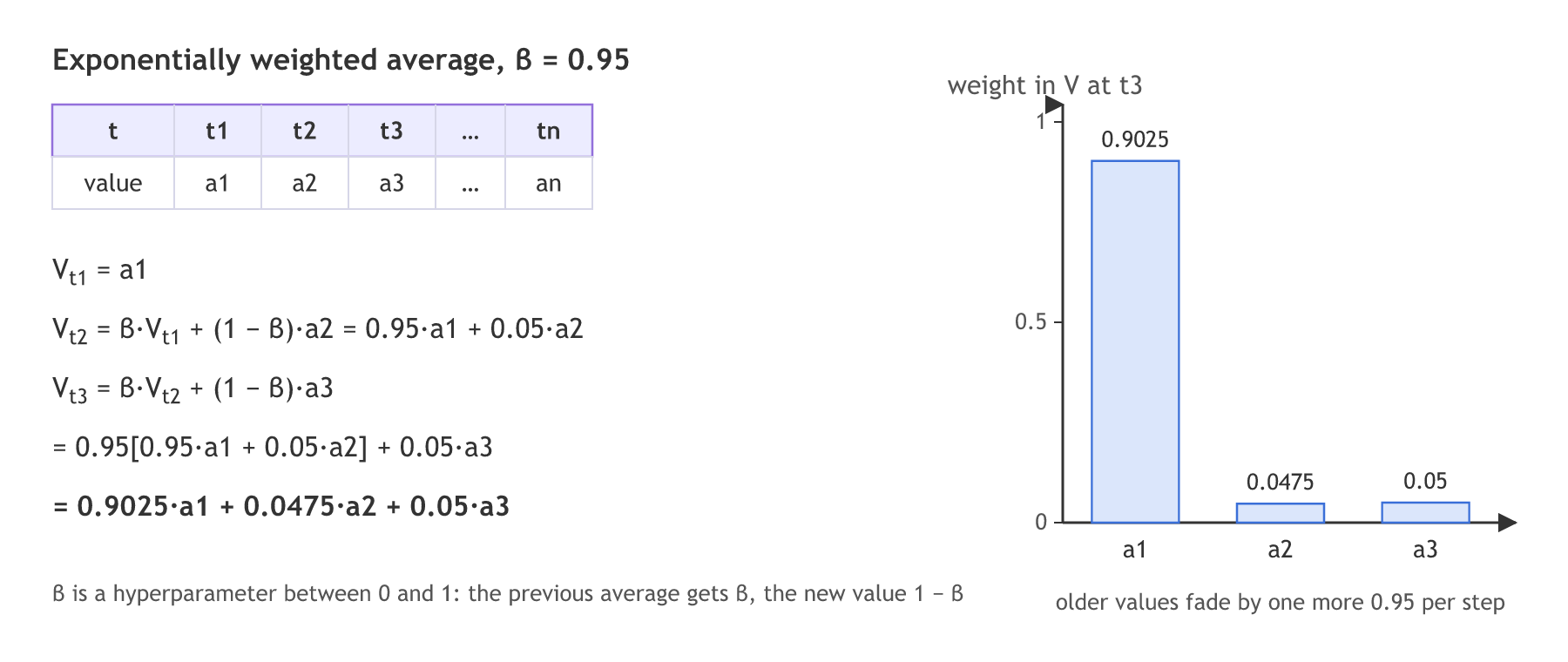
The exponentially weighted average (EWA) comes from time series, where models such as ARIMA and ARMA use it. Take values a1, a2, a3, … an at times t1, t2, t3, … tn. The average V starts at the first value, and each new V mixes the previous V with the new value:
β is a hyperparameter between 0 and 1 that says which value to focus on. With β = 0.95 the board gets Vt2 = 0.95·Vt1 + 0.05·a2: the previous average gets far more importance than the current value. Plot a1 and a2 and the average moves from a1 only a little towards a2, so the curve is smoothed. On a loss curve this means the path from t1 to t2 does not jump to wherever the newest gradient points; t3 and t4 are controlled the same way, and the path reaches the global minima with the noise removed.
The video goes on to Vt3 = β·Vt2 + (1 − β)·a3, where Vt2 is replaced by its whole expression. The notes in the materials write that out, which shows where the name comes from:
Every older value is multiplied by one more 0.95, so its weight shrinks exponentially with age. (The board starts the average at Vt1 = a1. Optimizers start it at 0 instead, which matters for Adam later.)
Applying the average to the gradient
Where does the average go? On the derivative of the loss. The update uses Vdw, the weighted average of the gradients, instead of the newest gradient on its own:
What this fixes, from the board:
- It reduces the noise: a gradient that points sideways for one batch is outvoted by the average of the recent ones.
- It works for mini-batch SGD, which is where the noise comes from.
- It gives quicker convergence, since the directions that agree from batch to batch add up while the zig-zags cancel.
The video also gives the interview version: if a model's training is very noisy, the answer is to bring a smoothing factor, momentum, into the optimizer. Interviewers rarely ask for the equations.
Looking ahead with Nesterov momentum
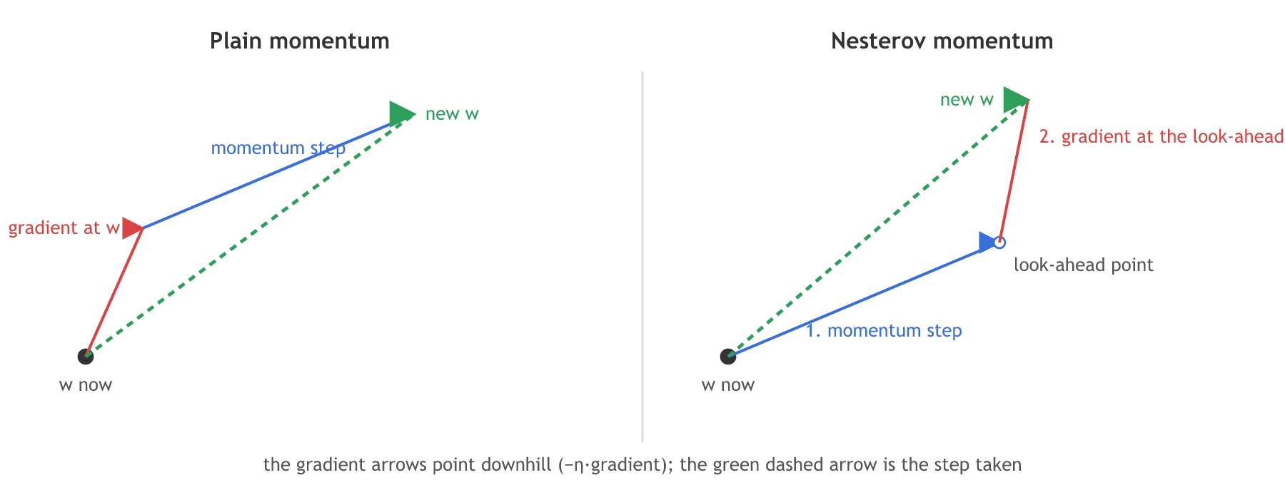
Nesterov accelerated gradient (NAG) is a small change that the video does not teach; the optimizer animation in the materials' notebook includes it. Plain momentum computes the gradient where the weights are now, then adds the momentum step. Nesterov first takes the momentum step to a look-ahead point, w − η·β·V, and computes the gradient there. If the momentum is about to overshoot the minimum, the look-ahead gradient already points back, so the correction comes one step earlier.
Smoothing a mini-batch path with momentum
The weights inside the average
To see the weights of a1, a2 and a3 inside V, feed the average unit vectors: then V's entries are the weights themselves.
import numpy as np

beta = 0.95
a = np.eye(3)                 # a1, a2, a3 as unit vectors, so V holds each value's weight
V = a[0]                      # V_t1 = a1
for t in (1, 2):
    V = beta * V + (1 - beta) * a[t]
print(f"V_t{t + 1} =", " + ".join(f"{c:.4f}·a{i + 1}" for i, c in enumerate(V) if c))V_t2 = 0.9500·a1 + 0.0500·a2 V_t3 = 0.9025·a1 + 0.0475·a2 + 0.0500·a3
The records and the momentum update
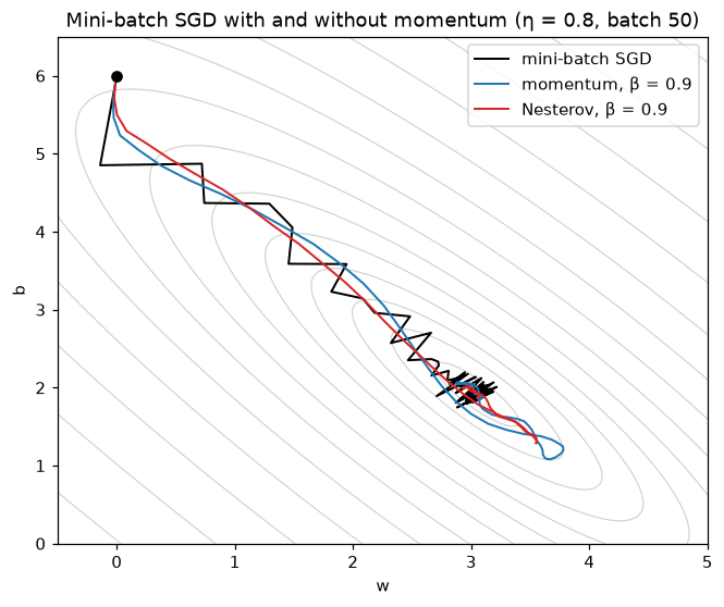
The same 1,000 records as before. To make the noise easy to see, the learning rate is high, η = 0.8, so plain mini-batch SGD zig-zags across the narrow valley of the cost. beta=0 turns the average off and gives plain mini-batch SGD; nesterov=True takes the gradient at the look-ahead point.
import numpy as np

rng = np.random.default_rng(42)
n = 1000                                     # 1,000 records stand in for the board's 1,000,000
x = rng.uniform(0, 2, n)
y = 3 * x + 2 + rng.normal(0, 0.5, n) # the true line has w = 3 and b = 2def gradients(w, b, xb, yb):
error = w * xb + b - yb # ŷ − y for every record in the batch
return np.mean(error * xb), np.mean(error) # ∂C/∂w and ∂C/∂b
def cost(w, b):
return np.mean((w * x + b - y) ** 2) / 2 # C = 1/(2n) Σ (y − ŷ)²def train(beta, lr=0.8, nesterov=False, epochs=5, batch_size=50):
order = np.random.default_rng(0)
w, b, v_w, v_b, path = 0.0, 6.0, 0.0, 0.0, [(0.0, 6.0)] # V_dw and V_db start at 0
for epoch in range(epochs):
idx = order.permutation(n)
for start in range(0, n, batch_size):
batch = idx[start:start + batch_size]
lw, lb = (w - lr * beta * v_w, b - lr * beta * v_b) if nesterov else (w, b)
gw, gb = gradients(lw, lb, x[batch], y[batch])
v_w = beta * v_w + (1 - beta) * gw # V_dw = β·V_dw + (1 − β)·∂L/∂w
v_b = beta * v_b + (1 - beta) * gb
w, b = w - lr * v_w, b - lr * v_b
path.append((w, b))
return np.array(path)Running plain, momentum and Nesterov
import matplotlib.pyplot as plt

fig, ax = plt.subplots(figsize=(7, 5.5))
W, B = np.meshgrid(np.linspace(-0.5, 5, 111), np.linspace(0, 6.5, 111))
ax.contour(W, B, np.vectorize(cost)(W, B), levels=np.geomspace(0.15, 20, 14), colors="lightgray", linewidths=0.8)
for name, beta, nest, color in [("mini-batch SGD", 0.0, False, "black"),
                                ("momentum, β = 0.9", 0.9, False, "tab:blue"),
                                ("Nesterov, β = 0.9", 0.9, True, "tab:red")]:
    path = train(beta, nesterov=nest)
    length = np.linalg.norm(np.diff(path, axis=0), axis=1).sum()
    print(f"{name:18} cost after 10 / 20 / 100 updates: "
          f"{cost(*path[10]):.3f} / {cost(*path[20]):.3f} / {cost(*path[100]):.4f}   path length {length:.2f}")
    ax.plot(path[:, 0], path[:, 1], color=color, lw=1.3, label=name)
ax.plot(0, 6, "ko"); ax.set_xlabel("w"); ax.set_ylabel("b")
ax.set_title("Mini-batch SGD with and without momentum (η = 0.8, batch 50)")
ax.legend(); plt.show()mini-batch SGD cost after 10 / 20 / 100 updates: 0.273 / 0.141 / 0.1282 path length 18.12 momentum, β = 0.9 cost after 10 / 20 / 100 updates: 0.724 / 0.173 / 0.1286 path length 8.57 Nesterov, β = 0.9 cost after 10 / 20 / 100 updates: 0.740 / 0.136 / 0.1282 path length 7.48
What the average changed
- Vt3 = 0.9025·a1 + 0.0475·a2 + 0.0500·a3, the board's expansion, and the three weights add up to 1.
- The path is far shorter with momentum. All three runs end at the same cost, but plain mini-batch SGD walks a much longer path to get there: the extra length is the zig-zag that the average cancels.
- Momentum starts slower. After 10 updates its cost is 0.724 against plain SGD's 0.273, because the average needs a few steps to build up from 0. Nesterov catches up by update 20 (0.136) and walks the shortest path of the three, 7.48 against 18.12 for plain mini-batch SGD.
- The zig-zags cancel, the agreeing direction stays. Across the valley the gradients flip sign from batch to batch and average out; along the valley they agree and add up.
Momentum in Keras
Keras puts momentum on its SGD optimizer:
import keras

opt = keras.optimizers.SGD(learning_rate=0.01, momentum=0.9)                 # momentum
opt = keras.optimizers.SGD(learning_rate=0.01, momentum=0.9, nesterov=True)  # Nesterov
model.compile(optimizer=opt, loss="binary_crossentropy", metrics=["accuracy"])
Keras writes the update without the (1 − β): velocity = momentum·velocity − η·gradient, then w = w + velocity. The direction is the same; once the velocity has built up, the steps come out 1/(1 − β) times larger, ten times for 0.9, so the same learning rate moves further than in the board's form.
Mini-batch SGD vs SGD with momentum
| Mini-batch SGD | SGD with momentum | |
|---|---|---|
| Step direction | the newest batch's gradient | the EWA of recent gradients, Vdw |
| Noise | zig-zags from batch to batch | smoothed |
| Extra setting | none | β (0.9 is common; the board uses 0.95) |
| First few steps | full size at once | slower while the average builds up |
| In Keras | SGD(momentum=0.0) | SGD(momentum=0.9) |
Where you use momentum
- Image models such as ResNets, which are often trained with SGD plus momentum 0.9 and a decaying learning rate.
- Long, narrow valleys in the cost, where plain SGD bounces between the walls.
- Inside Adam, which keeps the same average of gradients as its first ingredient.
nesterov=True.Related
- Previous: SGD and mini-batch gradient descent
- Next: Adagrad
- Change
beta = 0.95to 0.5 in the first example: Vt3 becomes 0.25·a1 + 0.25·a2 + 0.5·a3, so the newest value now counts most. - Change momentum's β from 0.9 to 0.99: the average reacts so slowly that the cost is still about 0.86 after 100 updates.
- Lower
lrto 0.2 intrain: plain mini-batch SGD stops zig-zagging, its path length falls to about 5.9, and momentum's advantage almost disappears.
You understood something today that you didn't yesterday.