Gradient descent
Gradient descent is an optimizer that updates every weight with wnew = wold − η·∂L/∂wold, using the whole training set for each update.
Last updated: 05 Oct, 2026 · NumPy
Choosing a loss function picked the number a network should make small. An optimizer is the rule that changes the weights to make it small. Gradient descent is the first one, and every optimizer in this part is a fix for one of its problems. For a refresher on the update rule itself on a single line, see Gradient descent in the Machine Learning course.
Updating the weights with gradient descent
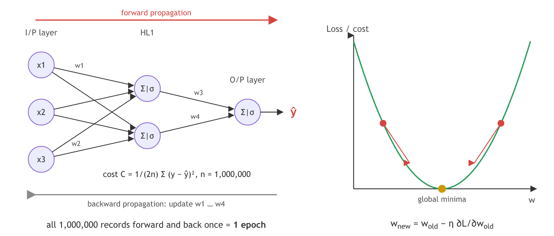
The board starts from the weight update formula that backpropagation uses:
Plot the loss against one weight w and the curve is a U. The bottom is the global minima. A point on either arm moves towards it: on the right arm the slope is positive and w decreases, on the left arm the slope is negative and w increases. The learning rate η sets how big each move is.
The network on the board has three inputs, one hidden layer (HL1) with two neurons and one output. Forward propagation multiplies the inputs by the weights, applies the activation and gives ŷ. The loss is the mean squared error, and backward propagation updates w1, w2, w3, w4 to make it smaller.
The video corrects its earlier sessions here: the MSE needs the n, so it is 1/(2n), not 1/2. The ½ is there so that the 2 from the square cancels when you take the derivative.
Defining an epoch
An epoch is one forward propagation plus one backward propagation over the training data. Say the dataset has 1,000,000 records. Gradient descent sends all one million through the forward pass at once, gets one ŷ for each, and the cost function's n is one million. Then backward propagation updates every weight once, based on that cost.
From here the video calls it the cost function rather than the loss, because it covers many records: the loss is the error of one record, the cost is the average over the n records in the pass.
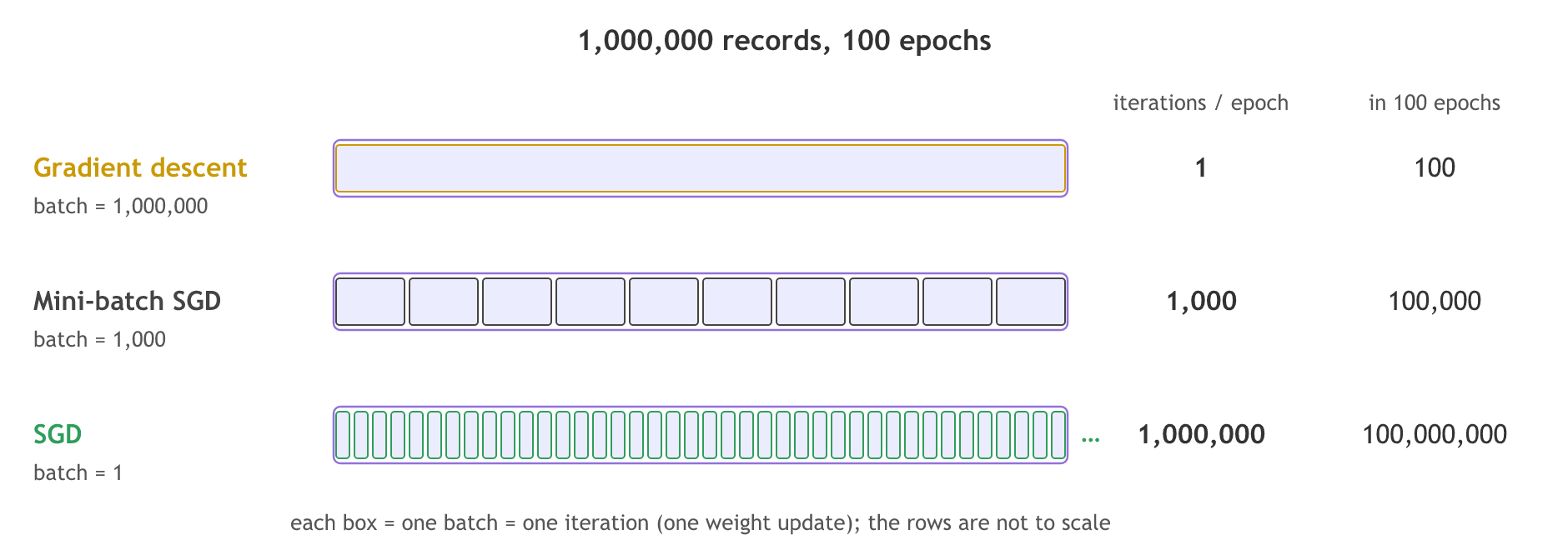
So in gradient descent one epoch is one weight update. Two more words come with the next optimizers. The batch size is how many records go through the network before one weight update; in gradient descent it is the whole dataset. An iteration is one such update, one batch forward and back, so iterations per epoch = records ÷ batch size. A network trains for many epochs; the video uses 100 as its example.
Why gradient descent is resource intensive
The video names one major disadvantage. To pass a million records in every epoch the machine must hold them all at once: it needs a huge RAM, and to compute that many forward passes in parallel it may need GPUs too. The upside is that each update uses the exact average over all records, so the path to the global minima is smooth and direct.
The question that leads to the next lesson: can an optimizer work well with fewer resources?
Counting iterations and running gradient descent
First the board's numbers. The same arithmetic gives the iterations for any batch size, and a rough memory figure shows why a million records is heavy: a record with 100 features stored as 4-byte floats is 400 bytes.
import math

records, epochs, features = 1_000_000, 100, 100
for name, batch_size in [("gradient descent", records), ("mini-batch SGD", 1000), ("SGD", 1)]:
    per_epoch = math.ceil(records / batch_size)          # iterations in one epoch
    print(f"{name:16} batch {batch_size:>9,}  per epoch {per_epoch:>9,}  in {epochs} epochs {per_epoch * epochs:>11,}")

batch_bytes = records * features * 4                     # float32 inputs of one gradient descent batch
print("inputs held for one gradient descent update:", batch_bytes / 1e6, "MB")gradient descent batch 1,000,000 per epoch 1 in 100 epochs 100 mini-batch SGD batch 1,000 per epoch 1,000 in 100 epochs 100,000 SGD batch 1 per epoch 1,000,000 in 100 epochs 100,000,000 inputs held for one gradient descent update: 400.0 MB
The records and the gradients
Now gradient descent for real, on a single neuron ŷ = w·x + b with no activation, which is linear regression. 1,000 records stand in for the million. The gradients are the derivatives of the 1/(2n) cost.
import numpy as np

rng = np.random.default_rng(42)
n = 1000                                     # 1,000 records stand in for the board's 1,000,000
x = rng.uniform(0, 2, n)
y = 3 * x + 2 + rng.normal(0, 0.5, n) # the true line has w = 3 and b = 2def gradients(w, b, xb, yb):
error = w * xb + b - yb # ŷ − y for every record in the batch
return np.mean(error * xb), np.mean(error) # ∂C/∂w and ∂C/∂b
def cost(w, b):
return np.mean((w * x + b - y) ** 2) / 2 # C = 1/(2n) Σ (y − ŷ)²One update per epoch
Every epoch passes all 1,000 records, so every epoch is one iteration:
w, b, lr = 0.0, 0.0, 0.5
for epoch in range(1, 101):
    gw, gb = gradients(w, b, x, y)           # all 1,000 records, one forward and backward pass
    w, b = w - lr * gw, b - lr * gb          # one weight update per epoch
    if epoch in (1, 2, 5, 10, 50, 100):
        print(f"epoch {epoch:3}: w = {w:.3f}  b = {b:.3f}  cost = {cost(w, b):.4f}")
print("records read:", 100 * n, " weight updates:", 100)epoch 1: w = 2.976 b = 2.472 cost = 0.2478 epoch 2: w = 2.747 b = 2.228 cost = 0.1439 epoch 5: w = 2.828 b = 2.173 cost = 0.1373 epoch 10: w = 2.903 b = 2.085 cost = 0.1322 epoch 50: w = 3.045 b = 1.917 cost = 0.1281 epoch 100: w = 3.051 b = 1.911 cost = 0.1281 records read: 100000 weight updates: 100
Reading the counts and the run
- Gradient descent does 1 iteration per epoch, 100 in 100 epochs. Mini-batch SGD with a batch of 1,000 does 1,000 per epoch, and SGD does 1,000,000 per epoch, 100,000,000 in 100 epochs: the board's numbers.
- 400 MB of inputs for one gradient descent update, before any hidden layer's outputs and gradients, which also scale with the batch. That is the huge RAM the board warns about.
- The cost falls every epoch and the weights settle near w = 3.05, b = 1.91, the best line for these noisy records (the true line is w = 3, b = 2; the noise moves the best fit a little).
- 100 updates cost 100,000 record reads. Each update looks at every record. The next optimizers trade this exactness for cheaper updates.
Epoch vs iteration vs batch size
| Batch size | Iteration | Epoch | |
|---|---|---|---|
| What it counts | records in one forward and backward pass | one weight update, one batch | one pass over every record |
| Gradient descent, 1,000,000 records | 1,000,000 | 1 per epoch | 1 weight update |
| Mini-batch SGD, batch 1,000 | 1,000 | 1,000 per epoch | 1,000 weight updates |
| Set in Keras by | batch_size in fit | records ÷ batch size, rounded up | epochs in fit |
Where you use gradient descent
- Small datasets that fit in memory, where a full pass is cheap and the smooth path is a bonus.
- Checking a new model: full-batch updates have no noise, so a cost that does not fall points to a bug, not to bad luck in a batch.
- As the base of every other optimizer: SGD, momentum, Adagrad, RMSprop and Adam all keep this update and change what goes into it.
model.fit uses mini-batches unless you pass batch_size=len(X), so a model trained with the optimizer called SGD is usually running mini-batch SGD.Related
- Previous: Choosing a loss function
- Next: SGD and mini-batch gradient descent
- Refresher: Gradient descent in the Machine Learning course
- Change
lrto 1.5 in the gradient descent run: the cost grows each epoch and the weights blow up, because the step overshoots the bottom of the U. - Set
features = 1000in the counting example: one gradient descent batch now needs 4,000 MB of inputs. - Change
lrto 0.05: after 100 epochs the cost is still 0.1324, above the 0.1281 that η = 0.5 reaches, because each of the 100 updates is a smaller step.
Every expert started right here.