Convolutional neural networks (CNN)
A convolutional neural network (CNN) is a neural network that slides small learned filters over an image to find edges, shapes and then whole objects, layer by layer.
Last updated: 05 Oct, 2026 · NumPy
The networks so far take one row of numbers per record, like the churn table in Building an ANN in Keras. A photo is a grid of pixels where neighbours belong together, and tasks such as image classification and object detection on images and video frames need a network that keeps that grid. That network is the CNN.
Comparing a CNN with the human brain
The video starts from how a person sees. One scene can hold a cat, a dog, a bicycle, a car and a human, and the brain takes in all of it at once: a person moving, an animal, a bird flying. The part doing this work is the cerebral cortex, and inside it, at the back of the brain, the visual cortex is responsible for seeing objects in an image or a video.
The board splits the visual cortex into layers V1 to V7, and the video says these layers are made up for the example: one sees moving objects, the next animals, the next maps the environment, and the last one gives the output. A CNN should do many stages of processing like this too.
The course notes give the real jobs: V1 picks up edges and the orientation of lines, and V2 differences in colour and complex patterns. The notes list V5 under object recognition, but V5 (also called MT) handles motion; recognising an object happens further along, in the inferotemporal (IT) cortex.
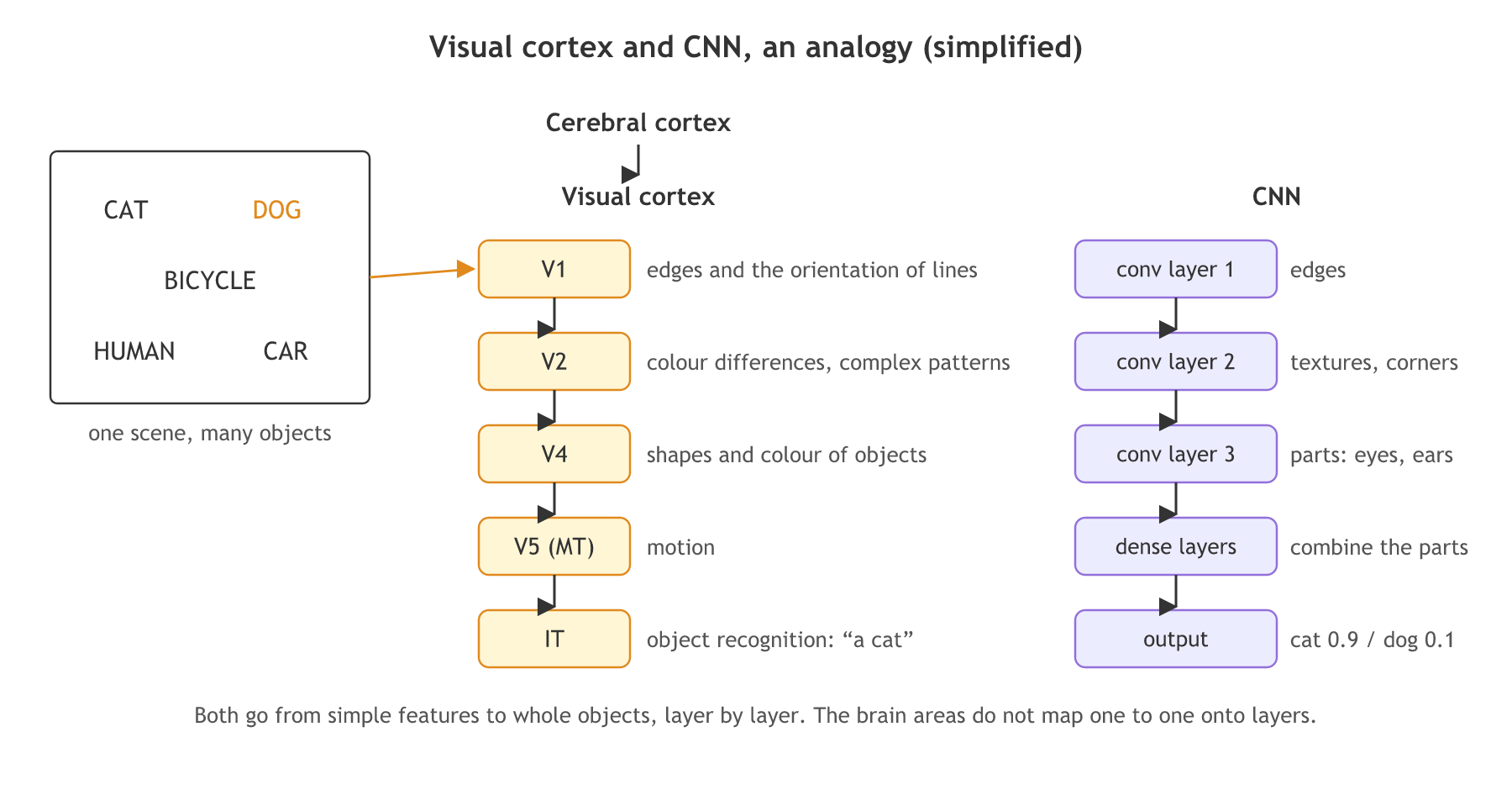
What carries over is the order: early stages see simple things and later stages combine them. A trained CNN's first layer responds to edges, deeper layers to textures and parts such as eyes or ears, and the dense layers at the end turn those parts into a class.
Representing images as pixels and channels
Before convolution comes the image itself. A photo is divided into pixels: the board draws a 5×5 pixel image, five pixels wide and five high. Each pixel holds a number from 0 to 255, where 0 is black and 255 is white, so one pixel may be 40, the next 0, another 255, 240 or 17. A black and white (grayscale) image has a single channel: one grid of numbers.
A colour photo from a phone or a DSLR is an RGB image with three channels, red, green and blue. Each channel is its own 5×5 grid with values from 0 to 255, and the three together can make every colour. The board writes its size as 5×5×3: height, width and the number of channels.
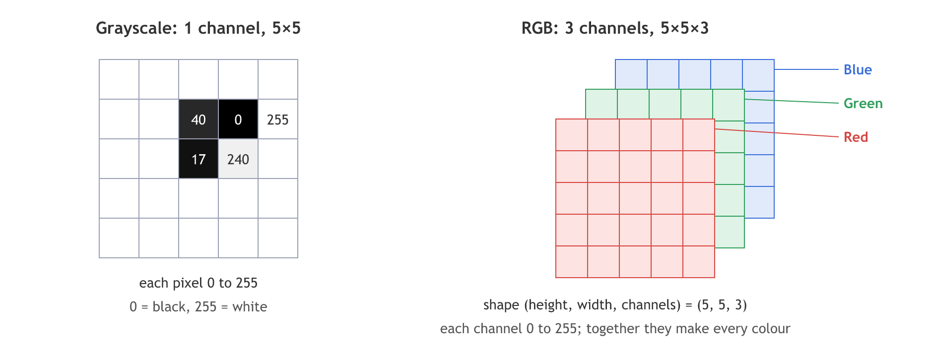
The same notation runs through the part: the CIFAR-10 photos in CNN in Keras are 32×32×3, and VGG16 in Transfer learning with VGG16 takes 224×224×3.
Storing images as NumPy arrays
In code an image is an array whose shape is (height, width, channels). A grayscale image may drop the channel axis.
A grayscale image
gray = np.zeros((5, 5), dtype=np.uint8)   # 5x5 pixels, one channel, all black
gray[1, 2:5] = [40, 0, 255]                # the board's values
gray[2, 2:4] = [17, 240]
An RGB image
The last axis holds the three channels. Filling channel 0 with 255 and leaving the others at 0 makes a pure red image.
rgb = np.zeros((5, 5, 3), dtype=np.uint8)  # 5x5 pixels, 3 channels
rgb[:, :, 0] = 255                          # red full, green and blue 0
Scaling the pixels to 0-1
Networks train better on small numbers, so the first step in the video's practical is dividing every pixel by 255.
scaled = gray / 255 # 0 stays 0, 255 becomes 1, 40 becomes 0.157Building the board's images in NumPy
The program builds both images, scales one, and counts how many weights a dense layer and a convolution layer would need on a 224×224 photo.
import numpy as np

gray = np.zeros((5, 5), dtype=np.uint8)        # 5x5, one channel
gray[1, 2:5] = [40, 0, 255]                     # the values on the board
gray[2, 2:4] = [17, 240]
print("grayscale shape:", gray.shape)
print(gray)

rgb = np.zeros((5, 5, 3), dtype=np.uint8)      # 5x5, three channels
rgb[:, :, 0] = 255                              # red channel full, green and blue 0
print("rgb shape:", rgb.shape, " pixel (0, 0):", rgb[0, 0])

scaled = gray / 255                             # 0-255 becomes 0-1
print("row 2 scaled:", np.round(scaled[1], 3))

values = 224 * 224 * 3
print("values in a 224x224 RGB image:", values)
print("Dense(64) weights on it:", values * 64 + 64)
print("Conv2D(64, 3x3) weights on it:", 3 * 3 * 3 * 64 + 64)grayscale shape: (5, 5) [[ 0 0 0 0 0] [ 0 0 40 0 255] [ 0 0 17 240 0] [ 0 0 0 0 0] [ 0 0 0 0 0]] rgb shape: (5, 5, 3) pixel (0, 0): [255 0 0] row 2 scaled: [0. 0. 0.157 0. 1. ] values in a 224x224 RGB image: 150528 Dense(64) weights on it: 9633856 Conv2D(64, 3x3) weights on it: 1792
What the arrays show
- The grayscale image has shape (5, 5): one number per pixel, with the board's 40, 0 and 255 in row 2 and 17 and 240 in row 3.
- The RGB image has shape (5, 5, 3), and its first pixel is [255 0 0]: full red, no green, no blue.
- Scaling turns 40 into 0.157 and 255 into 1.0; every value now lies between 0 and 1.
- A 224×224 photo holds 150,528 numbers. A dense layer of 64 neurons on it needs 9,633,856 weights, while 64 convolution filters of size 3×3×3 need 1,792, because each filter is reused at every position of the image.
CNN vs ANN
| ANN (dense layers) | CNN | |
|---|---|---|
| Input | one row of features | an image grid: height × width × channels |
| Weights | one per input per neuron | small filters shared across every position |
| Pixel neighbours | lost once the image is a flat row | kept: each filter looks at a small patch |
| First layer on 224×224×3 | Dense(64): 9,633,856 parameters | Conv2D(64, 3×3): 1,792 parameters |
| Typical tasks | tables: churn, prices | images and video frames |
Where you use CNNs
- Image classification: one label per photo, such as the ten CIFAR-10 classes or a diseased or fresh cotton leaf.
- Object detection: finding where each object sits in a photo or a video frame, with a box around it.
- Segmentation, which the course notes add: a label for every pixel, for example the road in a dashcam frame.
uint8, and uint8 arithmetic wraps around: np.uint8(250) + np.uint8(10) gives 4, not 260. Divide by 255 (which gives floats) before adding, subtracting or averaging pixel values.Related
- Previous: Black box vs white box models
- Next: Convolution and filters
- See also: Building an ANN in Keras
- Set
rgb[:, :, 1] = 255as well and printrgb[0, 0]: red plus green is yellow, [255 255 0]. - Change 224 to 32 (the CIFAR-10 size) and compare the Dense(64) and Conv2D(64) counts again.
- Run
np.uint8(250) + np.uint8(10)and thennp.uint8(250) / 255 + np.uint8(10) / 255to see the wrap-around and its fix.
Slow is fine. Stopping is the only problem.