Perceptron
A perceptron is the simplest neural network: one neuron that multiplies its inputs by weights, adds a bias, and passes the sum through an activation function to output a class, 0 or 1.
Last updated: 05 Oct, 2026 · NumPy
Every network later in the course, from the churn ANN to a CNN, is built from this unit repeated many times. The perceptron is the first neural network, and the video starts deep learning with it: first the single-layer network, then the multi-layer one.
Drawing a single-layer network
Draw three circles on the left: they are the input layer, one circle per input. Since this is a single-layer network, the next circle is hidden layer 1, and the last circle is the output layer. Every dot is connected to the next layer.
The example is a dataset that says whether a student passed. Each record has study, play and sleep hours, and the output is pass or fail. Two outcomes make it a binary classification problem, so pass is written as 1 and fail as 0:
- Studies 7 hours, plays 3, sleeps 7: pass (1).
- Studies 2 hours, plays 5, sleeps 8: fail (0).
- Studies 4 hours, plays 3, sleeps 7: pass (1).
The inputs go in record by record. Study is x1, play is x2 and sleep is x3, so the first pass feeds in 7, 3 and 7.
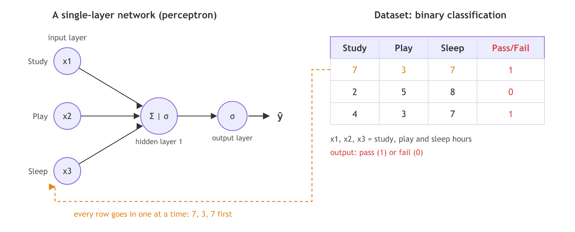
The board names the middle neuron "hidden layer 1" and adds a separate output neuron. A perceptron in its strict sense has no hidden layer: the inputs feed one neuron, and that neuron's output is the prediction. The two drawings compute the same kind of thing, a weighted sum and an activation; the code below uses the strict form.
Seeing, processing and training like a brain
The video maps the network onto how you recognise a camera. Your eyes are the input layer: the picture of the camera is the input signal. The signal goes to neurons in the hidden layer, and a biological neuron does some kind of signal processing. The output layer is the part at the back of the brain that decides what you are looking at: a camera, a television or a mobile phone. That final neuron is the output neuron.
A newborn baby who sees a camera for the first time cannot say what it is. Someone has to tell it, again and again: this is the camera, this is food, this is your bed, this is milk. After a few months it recognises the milk bottle and the phone. A neural network built from scratch is the same: it must be trained on inputs with their right outputs before it predicts anything useful. Like the brain, a network can have any number of hidden layers, and the signal passes from neuron to neuron through them.
Splitting the neuron into two steps
The notes for this topic list what a perceptron is made of, an input layer, a hidden layer, weights and an activation function, and split the neuron into two steps:
Step 2 passes z through an activation function, which turns it into the output. The notes draw two of them:
The notes write the sigmoid's rule as "1 if z > 0.5". The 0.5 threshold applies to the sigmoid's output σ(z), not to z: σ(z) ≥ 0.5 happens exactly when z ≥ 0, so both functions switch class at z = 0. The difference is that the step jumps from 0 to 1, while the sigmoid rises smoothly and gives a value in between that can be read as a probability.
Separating classes with a straight line
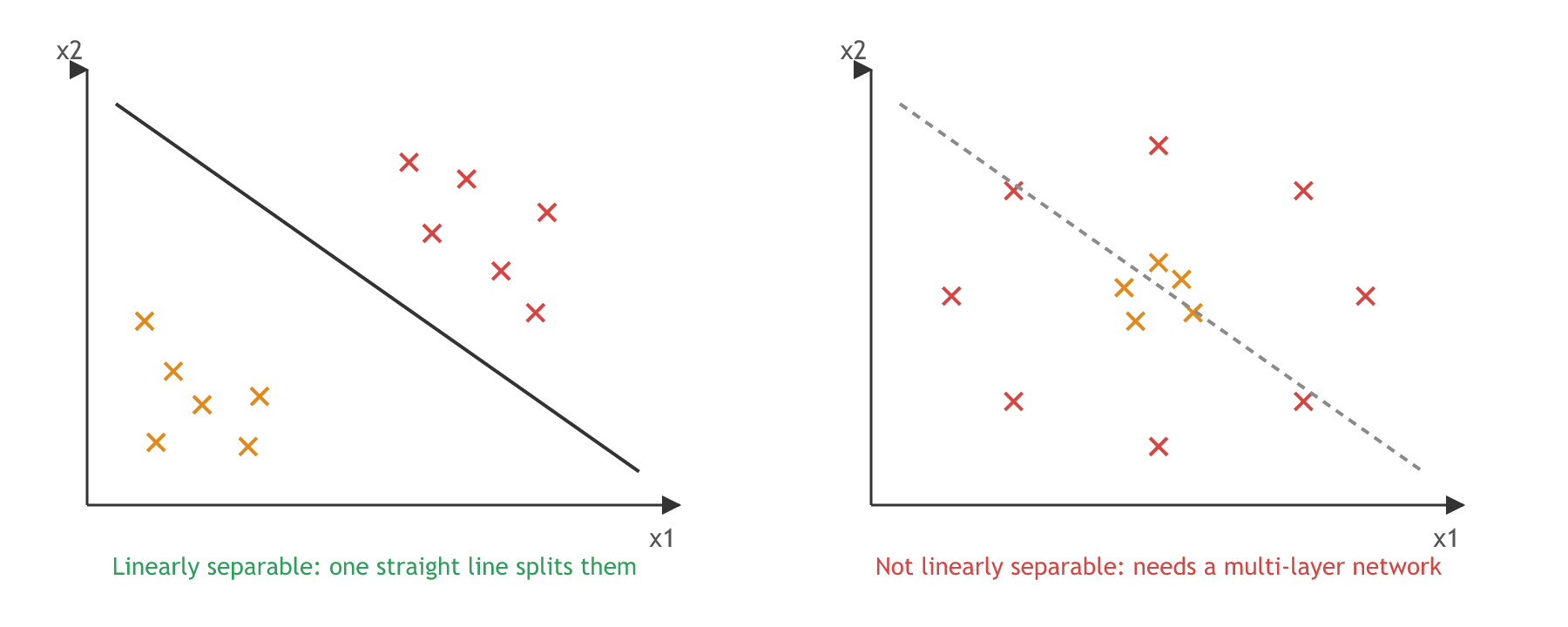
The rule z = w1x1 + w2x2 + b = 0 is a straight line (a plane with three inputs). Points on one side get class 1 and points on the other get class 0, so a perceptron is a linear classifier. If one straight line can split the two classes, the data is linearly separable and a perceptron can learn it. If one class surrounds the other, no line works, and the notes' answer is a multi-layer neural network.
Training a perceptron on the student table
The classic way to train one neuron with a step function is the perceptron learning rule: feed each record in, and when the prediction is wrong, move every weight by the learning rate × the error × that input. When the prediction is right, the error is 0 and nothing changes.
The student table
import numpy as np

# the video's student table: study, play and sleep hours, pass (1) or fail (0)
X = np.array([[7, 3, 7], [2, 5, 8], [4, 3, 7]])
y = np.array([1, 0, 1])
The step function and a prediction
def step(z):
    return (z > 0).astype(int)     # 1 when z > 0, else 0

def predict(X, w, b):
    return step(X @ w + b)          # step 1: sum, step 2: activation
The perceptron learning rule
def train(lr, epochs=3):
    w, b = np.zeros(3), 0.0                  # start from zero weights
    for epoch in range(1, epochs + 1):
        for xi, yi in zip(X, y):             # one record at a time
            error = yi - predict(xi, w, b)   # 0 when right, +1 or -1 when wrong
            w = w + lr * error * xi          # move the weights towards the answer
            b = b + lr * error
        print("epoch", epoch, "w", np.round(w, 2), "b", round(b, 2), "predictions", predict(X, w, b))
    return w, b
Learning the pass and fail rows
w, b = train(lr=0.1)

from sklearn.linear_model import Perceptron
clf = Perceptron(shuffle=False, random_state=0).fit(X, y)   # the same rule, learning rate 1
print("scikit-learn w", clf.coef_[0], "b", clf.intercept_[0], "predictions", clf.predict(X))epoch 1 w [ 0.5 -0.2 -0.1] b 0.0 predictions [1 0 1] epoch 2 w [ 0.5 -0.2 -0.1] b 0.0 predictions [1 0 1] epoch 3 w [ 0.5 -0.2 -0.1] b 0.0 predictions [1 0 1] scikit-learn w [ 5. -2. -1.] b 0.0 predictions [1 0 1]
Reading the training run
- Epoch 1 already fixes it. The first record (7, 3, 7) is predicted 0 by the zero weights, so w moves to 0.1 × 7, 3, 7. The second record (2, 5, 8) is then wrongly a pass, and w moves back by 0.1 × 2, 5, 8, giving 0.5, −0.2, −0.1.
- Epochs 2 and 3 change nothing: every prediction is right, every error is 0, so the rule stops moving the weights.
- scikit-learn's
Perceptronlands on 5, −2, −1: the same direction, ten times larger, because it uses a learning rate of 1. From zero weights, the learning rate only scales the line; it does not change which side each student falls on. - Study gets a positive weight, play and sleep negative ones: more study pushes towards a pass.
Comparing the step function and the sigmoid
import numpy as np
import matplotlib.pyplot as plt

z = np.linspace(-6, 6, 241)
fig, axes = plt.subplots(1, 2, figsize=(9, 3.4))
axes[0].plot(z, (z > 0).astype(int), color="tab:red")
axes[0].set_title("Step function: threshold at z = 0")
axes[1].plot(z, 1 / (1 + np.exp(-z)), color="tab:blue")
axes[1].axhline(0.5, color="gray", linestyle="--")
axes[1].set_title("Sigmoid: threshold at 0.5")
for ax in axes:
    ax.set_xlabel("z")
    ax.set_ylabel("output")
plt.tight_layout()

for v in [-0.1, 0.0, 0.1]:
    print(f"z = {v:5}: step {int(v > 0)}, sigmoid {1 / (1 + np.exp(-v)):.3f}")
plt.show()z = -0.1: step 0, sigmoid 0.475 z = 0.0: step 0, sigmoid 0.500 z = 0.1: step 1, sigmoid 0.525
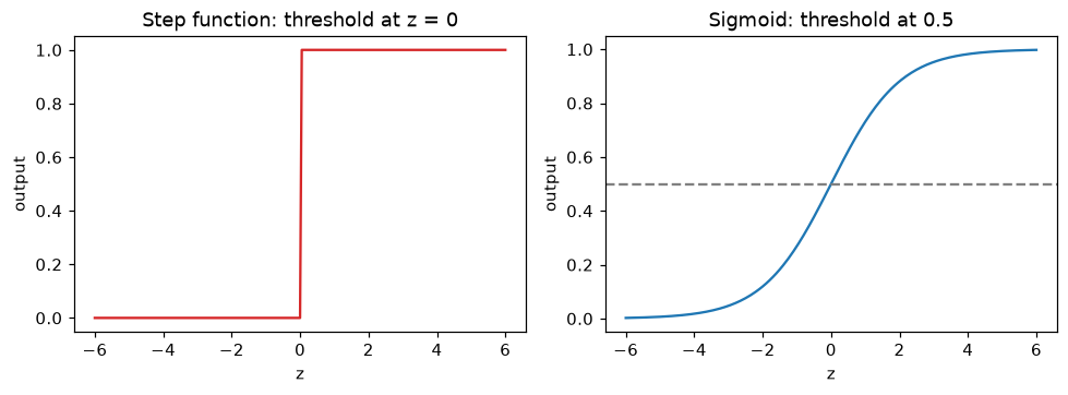
Near z = 0 the step function flips from 0 to 1 at once, while the sigmoid moves from 0.475 to 0.525. That smooth change is what lets a network learn by small adjustments, the subject of How a neural network learns.
Single-layer vs multi-layer perceptron
| Single-layer perceptron | Multi-layer perceptron (ANN) | |
|---|---|---|
| Layers | Inputs straight into one neuron | One or more hidden layers between inputs and outputs |
| Decision boundary | One straight line or plane | Curved, any shape with enough neurons |
| Data it can learn | Linearly separable only | Non-linearly separable too |
| Training | The perceptron learning rule | Forward propagation, loss, backpropagation, optimizer |
| Activation | Step function (or sigmoid) | Sigmoid, tanh, ReLU and others per layer |
Where you use a perceptron
- As the unit of every network. A Keras
Denselayer is a row of these neurons with a smooth activation in place of the step. - Simple linear yes/no rules on a few numeric inputs, such as pass or fail from study hours, where a straight line is enough.
- Interviews: "what is a perceptron and what can it not learn?" The answer is a linear classifier that fails on data that is not linearly separable.
Related
- Previous: Installing TensorFlow
- Next: Weights and bias
- See also: Logistic regression, the same neuron with a sigmoid, in the Machine Learning course
- Train on XOR: set
X = np.array([[0, 0], [0, 1], [1, 0], [1, 1]]),y = np.array([0, 1, 1, 0])andnp.zeros(2)insidetrain, then runtrain(lr=0.1, epochs=10). Every epoch ends on the same weights and the predictions 1, 1, 0, 0: the rule goes round in a circle and never reaches 0, 1, 1, 0. - Call
train(lr=1)and check that the hand-written rule now prints the same weights as scikit-learn. - Add a student who studies 3 hours, plays 6 and sleeps 6, predict with the trained
wandb, and say whether the answer matches your own guess.
This is what real progress feels like.