Loss and cost functions
A loss function is a formula that scores how wrong a neural network's prediction ŷ is for one record, and a cost function is the same score averaged over a batch of records.
Last updated: 05 Oct, 2026 · NumPy
After Forward propagation the network has a prediction ŷ, and the error y − ŷ is what backpropagation pushes down. The formula that turns that error into one number depends on the problem, and Choosing an activation function already tied the output layer to the problem type. This part picks the loss to go with it.
Splitting problems into regression and classification
An artificial neural network (ANN) solves two kinds of problems, and the board starts with one dataset for each.
- Regression: years of experience and degree give a salary. Someone with 10 years and a PhD earns a high salary, and salary is a continuous output.
- Classification: hours played and hours studied give the result. Playing 10 and studying 2 gives Fail, 4 and 3 Fail, 5 and 5 Maybe, 2 and 7 Pass. With Maybe in the column there are three classes, so this is a multi-class problem.
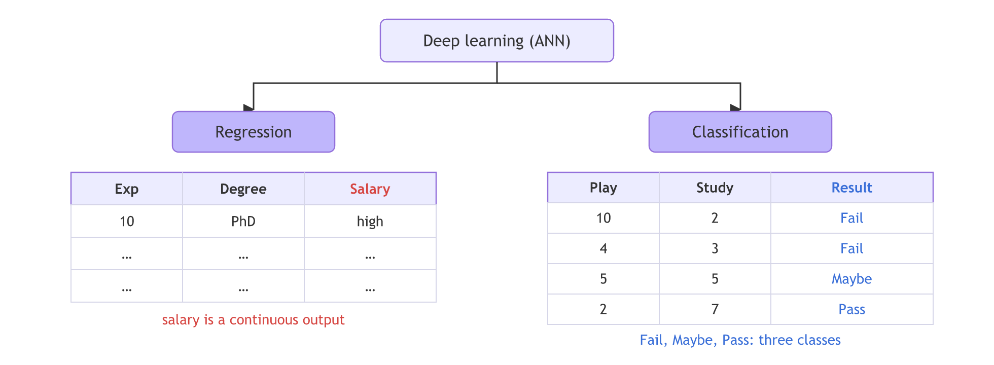
The rows are made up to show the shape of each dataset. Each kind of problem gets its own losses:
| Problem | Output | Loss functions |
|---|---|---|
| Regression | a continuous number | mean squared error (MSE), mean absolute error (MAE), Huber loss |
| Classification | a class | cross entropy: binary for two classes, categorical for more |
Computing the loss for one record
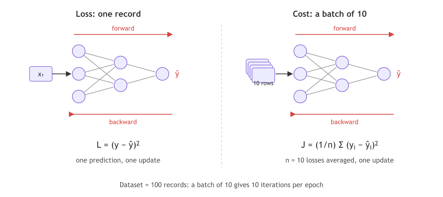
Take 100 records. The simplest training loop passes one record forward, computes ŷ, computes the loss and runs backpropagation, then moves to the next record. For a regression network the loss of that one record is the squared error:
Updating the weights after every single record is slow and noisy, which the video calls not an efficient scenario.
Averaging the loss over a batch into a cost
Instead, set a batch size, say 10. Each forward pass now carries 10 records, the loss is computed for each of them, and the 10 losses are combined into one number, the cost. In the video's words: in the loss function you provide one data point, in the cost function a batch of data points.
The board writes the cost as ½ Σ (y − ŷ)² with no 1/n; a cost is a mean over the batch, so it needs the 1/n (some books write 1/(2n) to tidy the derivative). The later notes write it with 1/n.
Counting batches, iterations and epochs
Right after the clip the video says a batch is passed in every epoch. One batch is one iteration, one weight update. An epoch is one full pass over all 100 records, so a batch of 10 means 10 iterations per epoch. Gradient descent builds on these three words.
Computing loss and cost in NumPy
The 100 records
A salary that grows by about 1.5 lakhs per year of experience, and a network whose predictions grow by 1.4:
import numpy as np

rng = np.random.default_rng(0)
experience = rng.uniform(0, 10, size=100).round(1)                     # 100 records
salary = (3 + 1.5 * experience + rng.normal(0, 1, size=100)).round(2)  # in lakhs
predicted = 3 + 1.4 * experience                                       # one network's ŷ
Loss of one record and cost of a batch
def loss(y, y_hat):
    return (y - y_hat) ** 2              # one record

def cost(y, y_hat):
    return np.mean((y - y_hat) ** 2)     # (1/n) Σ over a batch of n records
Comparing a mean with a half sum
print("loss, record 0:", round(loss(salary[0], predicted[0]), 3))
print("cost, records 0-9:", round(cost(salary[:10], predicted[:10]), 3))

for n in (10, 50, 100):
    half_sum = 0.5 * np.sum((salary[:n] - predicted[:n]) ** 2)
    print(f"batch of {n:3d}: half sum = {half_sum:7.3f}   mean = {cost(salary[:n], predicted[:n]):.3f}")

batch_size = 10
print("iterations per epoch:", len(salary) // batch_size)loss, record 0: 0.49 cost, records 0-9: 0.848 batch of 10: half sum = 4.241 mean = 0.848 batch of 50: half sum = 29.682 mean = 1.187 batch of 100: half sum = 61.464 mean = 1.229 iterations per epoch: 10
What the loss and cost printed
- Record 0 alone has a loss of 0.49: its salary is off by 0.7 lakhs, and 0.7² = 0.49.
- The first batch of 10 has a cost of 0.848, the average of 10 such losses. One weight update now uses all 10 records.
- The half sum grows with the batch: 4.241, 29.682, 61.464 for 10, 50 and 100 records, while the mean stays near 1 (0.848, 1.187, 1.229). With the mean, the size of the number does not depend on the batch size.
- 100 records with a batch of 10 give 10 iterations per epoch.
Loss function vs cost function
| Loss function | Cost function | |
|---|---|---|
| Input | one record | a batch of n records |
| Regression formula | (y − ŷ)² | (1/n) Σ (yᵢ − ŷᵢ)² |
| One update uses | one prediction | the batch's average error |
| Typical use | the formula you choose (MSE, cross entropy) | what the optimizer minimises during training |
Where you use loss and cost functions
- Compiling a model: the loss you pass to Keras is the per-record formula; Keras averages it over each batch, which is the cost.
- Reading a training log: the loss printed per epoch is a cost, averaged over batches, so it can be compared across batch sizes.
- Interviews: "what is the difference between a loss function and a cost function" is a standard question, and the answer is one record vs a batch.
Related
- Previous: Choosing an activation function
- Next: MSE, MAE and Huber loss
- Refresher: Cost function in the Machine Learning course
- Change
predictedto3 + 1.5 * experience: the cost of all 100 records drops to about 0.95, the noise left in the salaries, because the slope is now right. - Set
batch_size = 32:len(salary) // batch_sizeprints 3, and 4 records are left for a smaller last batch. - Print
cost(salary, predicted)for all 100 records and compare it with the mean of ten batch costs of 10 records each: they are equal.
Every expert started right here.