Adam optimizer
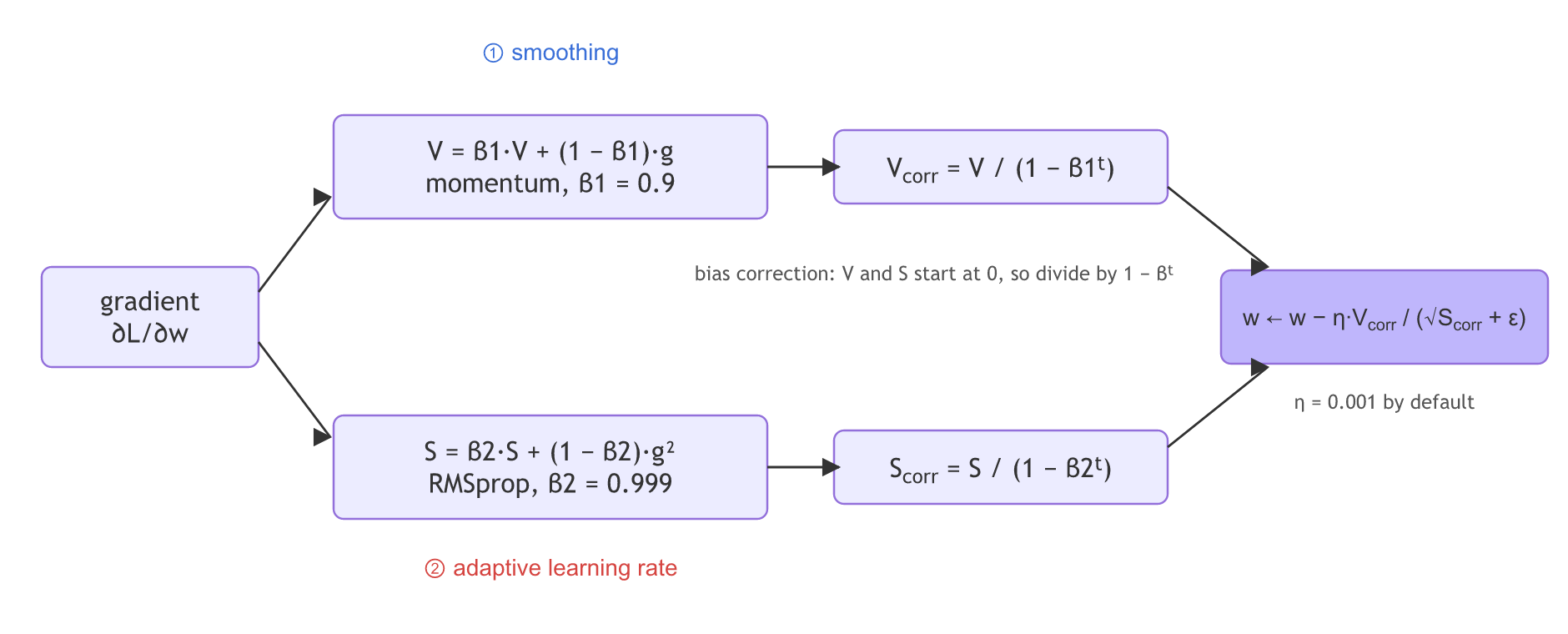
Adam (adaptive moment estimation) is an optimizer that combines momentum's average of the gradients with RMSprop's average of the squared gradients, so every step is both smoothed and scaled to its own learning rate.
Last updated: 05 Oct, 2026 · TensorFlow 2 / Keras
RMSprop and Adadelta made the learning rate adaptive, but the update still uses the raw gradient: the smoothing of SGD with momentum is missing. Adam puts the two together. The video calls it the best optimizer, the one most people use today.
Combining momentum and RMSprop
Adam keeps both averages, for the weights and for the bias. All four start at 0: Vdw = Vdb = Sdw = Sdb = 0. The update uses V (momentum) in place of the gradient, and η′ (RMSprop) in place of η:
This solves both problems at once: the smoothing of the path and the adaptive learning rate.
Three fixes to the board. The video first writes Vdw with a × before (1 − β) and corrects it to + in the clip. The board writes the bias update as bt = Wb,t−1 − η′Vdb; it is bt = bt−1 − η′b·Vdb, with η′b = η/√(Sdb + ε). And Sdb is set to 0 but never given its formula: it is the same EWA of (∂L/∂b)².
Adding β1, β2 and the bias correction
The board uses one β for both averages and stops there. The Adam paper (Kingma and Ba, 2015) adds two things:
- Two betas: β1 = 0.9 for the average of the gradients and β2 = 0.999 for the average of the squared gradients. The squared gradients are averaged over a much longer window.
- Bias correction: both averages start at 0, so for the first steps they are too small. With β1 = 0.9, the first V is 0.1·g, a tenth of the real gradient. Dividing by 1 − βt fixes that: at t = 1 it divides by 0.1 and gives back g, and as t grows 1 − βt goes to 1 and the correction fades.
The paper's default learning rate is η = 0.001, and Keras uses the same unless you set it. The ANN practical later in the video says Adam's default is 0.01; it is 0.001. Keras's other defaults are beta_1=0.9, beta_2=0.999 and epsilon=1e-7 (the paper uses 1e-8). Keras folds both corrections into the learning rate, η·√(1 − β2t)/(1 − β1t), and adds ε to √S before the correction, the paper's own efficient form; the steps are the same except that ε weighs a little more in the first few steps.
Running Adam in NumPy
The Adam loop
v_dw = s_dw = 0.0                                     # V_dw and S_dw start at 0
for t in range(1, steps + 1):
    g = gradient(w)
    v_dw = beta1 * v_dw + (1 - beta1) * g             # momentum: EWA of g
    s_dw = beta2 * s_dw + (1 - beta2) * g ** 2        # RMSprop: EWA of g²
    v_hat = v_dw / (1 - beta1 ** t)                   # bias correction
    s_hat = s_dw / (1 - beta2 ** t)
    w = w - lr * v_hat / (np.sqrt(s_hat) + eps)
The first steps with and without bias correction
A gradient of 2 at every step, the same each time, so the right V is 2 and the right S is 4:
import numpy as np

beta1, beta2, g = 0.9, 0.999, 2.0
v_dw = s_dw = 0.0
for t in range(1, 4):
    v_dw = beta1 * v_dw + (1 - beta1) * g
    s_dw = beta2 * s_dw + (1 - beta2) * g ** 2
    v_hat, s_hat = v_dw / (1 - beta1 ** t), s_dw / (1 - beta2 ** t)
    print(f"t = {t}: V = {v_dw:.3f} -> {v_hat:.3f}   S = {s_dw:.5f} -> {s_hat:.3f}"
f" step / η: {v_dw / np.sqrt(s_dw):.3f} uncorrected, {v_hat / np.sqrt(s_hat):.3f} corrected")t = 1: V = 0.200 -> 2.000 S = 0.00400 -> 4.000 step / η: 3.162 uncorrected, 1.000 corrected t = 2: V = 0.380 -> 2.000 S = 0.00800 -> 4.000 step / η: 4.250 uncorrected, 1.000 corrected t = 3: V = 0.542 -> 2.000 S = 0.01199 -> 4.000 step / η: 4.950 uncorrected, 1.000 corrected
Comparing the optimizers on one function
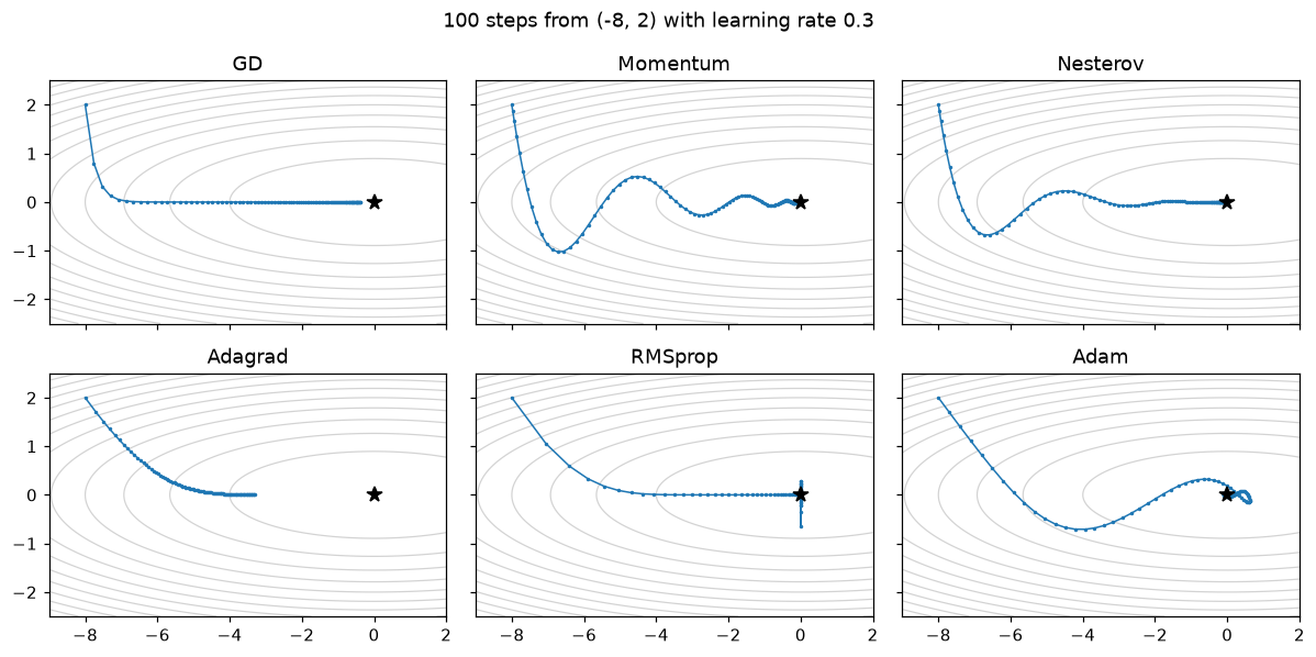
One function for every optimizer in this part: a long, narrow bowl f(w1, w2) = w1²/20 + w2², steep across w2 and flat along w1, with its minimum at (0, 0). Every optimizer starts at (−8, 2) with the same learning rate, 0.3, for 100 steps; momentum, Nesterov and RMSprop use β = 0.9, Adam uses β1 = 0.9 and β2 = 0.999.
The bowl
import numpy as np

def f(w):
    return w[0] ** 2 / 20 + w[1] ** 2                 # a long, narrow bowl, minimum at (0, 0)

def grad(w):
    return np.array([w[0] / 10, 2 * w[1]])
Six optimizers in one function
Each branch is one update rule from this part. Momentum and Nesterov share the average, Adagrad and RMSprop differ only in the line for s, and Adam uses both v and s with the bias correction.
def run(name, lr=0.3, steps=100, beta=0.9, b1=0.9, b2=0.999, eps=1e-8):
    w, v, s, path = np.array([-8.0, 2.0]), np.zeros(2), np.zeros(2), []
    for t in range(1, steps + 1):
        path.append(w.copy())
        g = grad(w - lr * beta * v) if name == "Nesterov" else grad(w)
        if name == "GD":         w = w - lr * g
        elif name in ("Momentum", "Nesterov"):
            v = beta * v + (1 - beta) * g; w = w - lr * v
        elif name == "Adagrad":  s = s + g ** 2;                 w = w - lr * g / np.sqrt(s + eps)
        elif name == "RMSprop":  s = beta * s + (1 - beta) * g ** 2; w = w - lr * g / np.sqrt(s + eps)
        elif name == "Adam":
            v = b1 * v + (1 - b1) * g; s = b2 * s + (1 - b2) * g ** 2
            w = w - lr * (v / (1 - b1 ** t)) / (np.sqrt(s / (1 - b2 ** t)) + eps)
    path.append(w.copy())
    return np.array(path)
Racing the six
import matplotlib.pyplot as plt

names = ["GD", "Momentum", "Nesterov", "Adagrad", "RMSprop", "Adam"]
fig, axes = plt.subplots(2, 3, figsize=(11, 5.5), sharex=True, sharey=True)
W1, W2 = np.meshgrid(np.linspace(-9, 2, 120), np.linspace(-2.5, 2.5, 120))
for name, ax in zip(names, axes.flat):
    path = run(name)
    print(f"{name:8} f after 25 steps {f(path[25]):.4f}   after 100 steps {f(path[100]):.5f}"
          f"   ends at ({path[100, 0]:.3f}, {path[100, 1]:.3f})")
    ax.contour(W1, W2, f([W1, W2]), levels=12, colors="lightgray", linewidths=0.8)
    ax.plot(path[:, 0], path[:, 1], ".-", ms=2.5, lw=1)
    ax.plot(0, 0, "k*", ms=9); ax.set_title(name)
fig.suptitle("100 steps from (-8, 2) with learning rate 0.3"); plt.tight_layout(); plt.show()GD f after 25 steps 0.6978 after 100 steps 0.00724 ends at (-0.380, 0.000) Momentum f after 25 steps 1.2990 after 100 steps 0.00042 ends at (-0.083, 0.009) Nesterov f after 25 steps 1.0958 after 100 steps 0.00078 ends at (-0.125, 0.000) Adagrad f after 25 steps 1.6313 after 100 steps 0.54370 ends at (-3.298, 0.002) RMSprop f after 25 steps 0.0357 after 100 steps 0.03188 ends at (-0.000, 0.179) Adam f after 25 steps 0.1244 after 100 steps 0.00002 ends at (-0.019, 0.001)
Reading the race
- Bias correction keeps the first step honest. Uncorrected, V is 0.2 and S is 0.004, so the first step is 3.162·η, three times too big; corrected, V = 2 and S = 4 and the step is exactly 1·η.
- Adam ends closest to the minimum after 100 steps. Its step is scaled per weight, so the flat w1 direction moves as fast as the steep w2 direction.
- Gradient descent is slow along the flat direction, where the gradient w1/10 is small: after 100 steps it is still at w1 ≈ −0.38.
- Momentum and Nesterov are behind gradient descent after 25 steps (the average is still building up) and well ahead after 100.
- Adagrad stops well short at w1 ≈ −3.3: its learning rate has shrunk, as in the Adagrad lesson.
- RMSprop gets w1 to 0 but bounces in w2 at about ±0.18: its steps keep their size near the minimum and its gradient is not smoothed. Adam's momentum average is what damps that bounce.
- One function, one learning rate. With each learning rate tuned separately the order can change; on this bowl a well-tuned gradient descent does very well. The race shows the behaviour each rule was built for, not a ranking for every problem.
Adam in Keras
import keras

opt = keras.optimizers.Adam(learning_rate=0.001, beta_1=0.9, beta_2=0.999)
model.compile(optimizer=opt, loss="binary_crossentropy", metrics=["accuracy"])
model.compile(optimizer="adam", loss="binary_crossentropy")   # the same, by name
Choosing an optimizer
| Optimizer | What it fixes | What is left | Reach for it when |
|---|---|---|---|
| Gradient descent | exact gradient, smooth path | huge RAM per update | the data is small |
| SGD | memory: one record per update | very noisy, slow | data arrives one record at a time |
| Mini-batch SGD | memory and noise balanced | some noise; one fixed η | the baseline for any network |
| SGD with momentum / Nesterov | noise: EWA of gradients | one fixed η for all weights | image models trained long, with a schedule |
| Adagrad | per-weight adaptive η | η′ shrinks towards 0 | sparse features, short training |
| RMSprop / Adadelta | η′ stays under control | no smoothing of the gradient | recurrent and reinforcement learning models |
| Adam | smoothing and adaptive η together | can generalise slightly worse than tuned SGD | the default first choice |
Where you use Adam
- The first run of almost any network: Adam with η = 0.001 trains most models without tuning.
- Transformers and language models, trained with Adam or its variant AdamW (weight decay kept apart from the gradient).
- Sparse or noisy gradients, where the per-weight scaling and the averaging both help. The video also names Adamax, a variant built on the same idea.
learning_rate explicitly in keras.optimizers.Adam so the value is visible in your code.Related
- Previous: RMSprop and Adadelta
- Next: Weight initialization
- Reference: Keras Adam
- In the race, change
lr=0.3tolr=0.03: no optimizer gets near the minimum in 100 steps, and RMSprop now ends lowest. The learning rate matters as much as the rule. - In the bias-correction example, set
beta1 = 0.99: the uncorrected V at t = 1 is now only 0.02, a hundredth of the gradient. - Remove the bias correction from Adam in
runby dividing by 1 instead of1 - b1 ** tand1 - b2 ** t, and compare its first steps with the corrected run.
Every expert started right here.