Binary cross-entropy
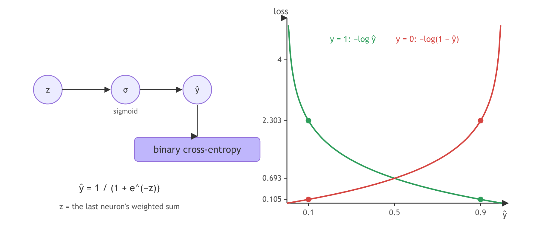
Binary cross-entropy is a classification loss function that scores a predicted probability ŷ against a label of 0 or 1: it costs −log ŷ when the label is 1 and −log(1 − ŷ) when the label is 0.
Last updated: 05 Oct, 2026 · TensorFlow 2 / Keras
The regression losses in MSE, MAE and Huber loss measure a distance between numbers. A classifier outputs a probability, and its loss comes from the cross entropy family. Binary cross-entropy is the same log loss that logistic regression uses, covered in Log loss.
The board's box writes ŷ = 1/(1 + e^−x); the sigmoid is applied to the last neuron's weighted sum z, so ŷ = 1/(1 + e^−z).
Splitting cross entropy into binary and categorical
- Binary cross-entropy for binary classification: two classes, such as pass or fail, spam or not spam.
- Categorical cross-entropy for multi-class classification: three or more classes, covered in Categorical cross-entropy.
Writing the binary cross-entropy formula
y is the true label, 0 or 1, and ŷ is the predicted probability that the label is 1. For the cost of a batch the video adds a sum over the records i = 1 to n; dividing that sum by n makes it the average.
Reading the two branches
Put each label into the formula. With y = 0 the first term is 0 · log ŷ = 0 and 1 − y = 1, so only −log(1 − ŷ) is left. With y = 1 the second term vanishes and −log ŷ is left:
The log is the natural log. A confident right answer costs almost nothing, and a confident wrong answer costs a lot:
| ŷ | Loss if y = 1: −ln ŷ | Loss if y = 0: −ln(1 − ŷ) |
|---|---|---|
| 0.9 | 0.105 | 2.303 |
| 0.5 | 0.693 | 0.693 |
| 0.1 | 2.303 | 0.105 |
Getting ŷ from the sigmoid in the last layer
The video's question is how ŷ is calculated. The output layer of a binary classifier has one neuron with the sigmoid activation, so ŷ = σ(z) lies between 0 and 1. Binary cross-entropy is applied on top of it, and backpropagation starts from that loss.
Computing binary cross-entropy in NumPy
The sigmoid and the loss
import numpy as np

def sigmoid(z):
    return 1 / (1 + np.exp(-z))

def bce(y, y_hat):
    return -(y * np.log(y_hat) + (1 - y) * np.log(1 - y_hat))
Four records through the last neuron
z = np.array([2.2, -1.4, 0.0, -3.0])    # the last neuron's weighted sums
y = np.array([1, 0, 1, 1])              # true labels
y_hat = sigmoid(z)
print("y_hat:", y_hat.round(3))
print("loss :", bce(y, y_hat).round(3))
print("cost :", round(bce(y, y_hat).mean(), 3))
for p in (0.9, 0.5, 0.1):
print(f"y_hat = {p}: loss if y = 1 is {bce(1, p):.3f}, if y = 0 is {bce(0, p):.3f}")y_hat: [0.9 0.198 0.5 0.047] loss : [0.105 0.22 0.693 3.049] cost : 1.017 y_hat = 0.9: loss if y = 1 is 0.105, if y = 0 is 2.303 y_hat = 0.5: loss if y = 1 is 0.693, if y = 0 is 0.693 y_hat = 0.1: loss if y = 1 is 2.303, if y = 0 is 0.105
A very confident wrong answer
With z = 40 the sigmoid rounds to exactly 1.0 in floating point, so 1 − ŷ is 0 and log 0 is minus infinity. NumPy prints a divide warning and the loss comes out as inf, which would break training. Writing the loss directly in terms of z avoids forming 1 − ŷ:
def bce_from_logits(y, z):
    # the same loss written with z, never forming 1 - ŷ
return np.maximum(z, 0) - z * y + np.log1p(np.exp(-np.abs(z)))z, y = 40.0, 0 # very confident, and wrong
print("from y_hat:", bce(y, sigmoid(z)))
print("from z :", bce_from_logits(y, z))
print("the four records from z:", bce_from_logits(np.array([1, 0, 1, 1]), np.array([2.2, -1.4, 0.0, -3.0])).round(3))from y_hat: inf from z : 40.0 the four records from z: [0.105 0.22 0.693 3.049]
The slope a wrong record sends back
Why not train a classifier with MSE on ŷ? Compare the slope of each loss with respect to z for a record that is confidently wrong:
z, y = -6.0, 1                          # confidently wrong: y_hat is about 0.0025
s = sigmoid(z)
print("dL/dz, binary cross-entropy:", round(s - y, 4))
print("dL/dz, squared error :", round(2 * (s - y) * s * (1 - s), 4))dL/dz, binary cross-entropy: -0.9975 dL/dz, squared error : -0.0049
What the losses printed
- The four records get ŷ = 0.9, 0.198, 0.5 and 0.047. The last one is labelled 1 but predicted 0.047, so it costs 3.049, far more than the others (0.105, 0.22, 0.693). The cost is their mean, 1.017.
- The table values come out of the same function: 0.105, 0.693 and 2.303, mirrored between the two labels.
- From ŷ, z = 40 gives inf; from z it gives 40.0, the correct loss (about z for a large wrong z). The four records give the same losses from z as from ŷ.
- The slope for a wrong record is −0.9975 with binary cross-entropy and −0.0049 with squared error. The sigmoid's slope σ(1 − σ) is tiny at z = −6 and multiplies the squared error's gradient, so the network barely learns from its worst mistakes. With binary cross-entropy the slope is ŷ − y, large exactly when the prediction is wrong.
Binary cross-entropy in Keras
The output layer gets one neuron with a sigmoid, and the loss is named in compile. With from_logits=True the last layer has no activation and the loss works from z, the stable form above:
import keras
from keras import layers

model = keras.Sequential([keras.Input(shape=(3,)),
                          layers.Dense(4, activation="relu"),
                          layers.Dense(1, activation="sigmoid")])   # ŷ between 0 and 1
model.compile(optimizer="adam", loss="binary_crossentropy", metrics=["accuracy"])

# or: no sigmoid in the last layer, and the loss applies it to z
# layers.Dense(1) with loss=keras.losses.BinaryCrossentropy(from_logits=True)
Binary cross-entropy vs MSE for classification
| Binary cross-entropy | MSE on a sigmoid output | |
|---|---|---|
| Loss for y = 1, ŷ = 0.1 | 2.303 | 0.81 |
| Slope with respect to z | ŷ − y | 2(ŷ − y) · ŷ(1 − ŷ) |
| Confidently wrong record | large slope, fast correction | slope near 0, slow learning |
| Shape over a logistic model's weights | convex | not convex |
Where you use binary cross-entropy
- Yes or no outputs: customer churn, spam detection, pass or fail, with one sigmoid neuron at the end.
- Multi-label outputs: one sigmoid per label (a photo can contain a cat and a dog), with a binary cross-entropy for each label; see Choosing a loss function.
- Imbalanced data: the same loss with class weights, so the rare class counts more.
from_logits=True the last layer must have no activation; a sigmoid layer plus from_logits=True squeezes the output again, and the loss and gradients are wrong. Training does not stop: at most a warning is printed, on the TensorFlow backend.Related
- Previous: MSE, MAE and Huber loss
- Next: Categorical cross-entropy
- Refresher: Log loss in the Machine Learning course
- Reference: Probabilistic losses in the Keras documentation
- Change the last label in
yfrom 1 to 0: that record's loss drops from 3.049 to about 0.049. - Call
bce(1, 1e-12)andbce_from_logits(1, -27.6): both give about 27.6, the loss for a near-zero probability. - Set
z = 6.0withy = 1in the slope check: both slopes are close to 0, because the prediction is right.
You understood something today that you didn't yesterday.