Transfer learning with VGG16
Transfer learning is a technique that reuses a network already trained on a large dataset, here VGG16 trained on ImageNet, as a fixed feature extractor and trains only a small new output layer for your own classes.
Last updated: 05 Oct, 2026 · TensorFlow 2 / Keras
The CIFAR-10 model in CNN in Keras learned all its filters from 50,000 images. With a few thousand images that is not enough, but the filters a big network learned on ImageNet's 1.2 million photos (edges, textures, parts) suit most photos. The video says that the number of layers is learned from transfer learning and the ImageNet competition, and promises transfer learning for a later session. The Transfer Learning VGG16 notebook in the Advanced-CNN-Architectures materials repo does it on cotton plant disease photos with 4 classes, run on TensorFlow 2.2.0 in September 2020. Its cells and saved outputs follow.
Loading VGG16 without its top
VGG16 is a CNN of 13 convolution layers, all 3×3 with same padding, in five blocks separated by 2×2 max pooling, followed by three dense layers. include_top=False drops the three dense layers, which were built for ImageNet's 1,000 classes, and keeps the convolutional base. weights='imagenet' downloads the trained filters (58,889,256 bytes). Every image is resized to 224×224, and IMAGE_SIZE + [3] adds the 3 RGB channels.
The notebook first prints its TensorFlow version and then imports the layers, the Model class, VGG16 and glob. Some imports, such as VGG19, Lambda and Sequential, are never used.
import tensorflow as tf
print(tf.__version__)2.2.0
# import the libraries as shown below

from tensorflow.keras.layers import Input, Lambda, Dense, Flatten
from tensorflow.keras.models import Model
from tensorflow.keras.applications.vgg16 import VGG16
from tensorflow.keras.applications.vgg19 import VGG19
from tensorflow.keras.preprocessing import image
from tensorflow.keras.preprocessing.image import ImageDataGenerator,load_img
from tensorflow.keras.models import Sequential
import numpy as np
from glob import glob
#import matplotlib.pyplot as plt# re-size all the images to this
IMAGE_SIZE = [224, 224]
train_path = 'Datasets/train'
valid_path = 'Datasets/test'# Import the VGG16 library as shown below and add preprocessing layer to the front of VGG
# Here we will be using imagenet weights
vgg16 = VGG16(input_shape=IMAGE_SIZE + [3], weights='imagenet', include_top=False)Downloading data from https://storage.googleapis.com/tensorflow/keras-applications/vgg16/vgg16_weights_tf_dim_ordering_tf_kernels_notop.h5 58892288/58889256 [==============================] - 3s 0us/step
Freezing the convolutional base
Setting trainable = False on every layer of the base means backpropagation leaves the ImageNet filters as they are; only the layers added next will learn.
# don't train existing weights
for layer in vgg16.layers:
    layer.trainable = False
Adding a new classification head
The number of classes is read from the training folders: one folder per class.
  # useful for getting number of output classes
folders = glob('Datasets/train/*')folders['Datasets/train\\diseased cotton leaf', 'Datasets/train\\diseased cotton plant', 'Datasets/train\\fresh cotton leaf', 'Datasets/train\\fresh cotton plant']
The head is a Flatten on the base's output and a Dense layer with one softmax unit per folder. Keras' functional API joins them: Model(inputs=vgg16.input, outputs=prediction).
# our layers - you can add more if you want
x = Flatten()(vgg16.output)

prediction = Dense(len(folders), activation='softmax')(x)

# create a model object
model = Model(inputs=vgg16.input, outputs=prediction)# view the structure of the model
model.summary()Model: "model" _________________________________________________________________ Layer (type) Output Shape Param # ================================================================= input_1 (InputLayer) [(None, 224, 224, 3)] 0 _________________________________________________________________ block1_conv1 (Conv2D) (None, 224, 224, 64) 1792 _________________________________________________________________ block1_conv2 (Conv2D) (None, 224, 224, 64) 36928 _________________________________________________________________ block1_pool (MaxPooling2D) (None, 112, 112, 64) 0 _________________________________________________________________ block2_conv1 (Conv2D) (None, 112, 112, 128) 73856 _________________________________________________________________ block2_conv2 (Conv2D) (None, 112, 112, 128) 147584 _________________________________________________________________ block2_pool (MaxPooling2D) (None, 56, 56, 128) 0 _________________________________________________________________ block3_conv1 (Conv2D) (None, 56, 56, 256) 295168 _________________________________________________________________ block3_conv2 (Conv2D) (None, 56, 56, 256) 590080 _________________________________________________________________ block3_conv3 (Conv2D) (None, 56, 56, 256) 590080 _________________________________________________________________ block3_pool (MaxPooling2D) (None, 28, 28, 256) 0 _________________________________________________________________ block4_conv1 (Conv2D) (None, 28, 28, 512) 1180160 _________________________________________________________________ block4_conv2 (Conv2D) (None, 28, 28, 512) 2359808 _________________________________________________________________ block4_conv3 (Conv2D) (None, 28, 28, 512) 2359808 _________________________________________________________________ block4_pool (MaxPooling2D) (None, 14, 14, 512) 0 _________________________________________________________________ block5_conv1 (Conv2D) (None, 14, 14, 512) 2359808 _________________________________________________________________ block5_conv2 (Conv2D) (None, 14, 14, 512) 2359808 _________________________________________________________________ block5_conv3 (Conv2D) (None, 14, 14, 512) 2359808 _________________________________________________________________ block5_pool (MaxPooling2D) (None, 7, 7, 512) 0 _________________________________________________________________ flatten (Flatten) (None, 25088) 0 _________________________________________________________________ dense (Dense) (None, 4) 100356 ================================================================= Total params: 14,815,044 Trainable params: 100,356 Non-trainable params: 14,714,688 _________________________________________________________________
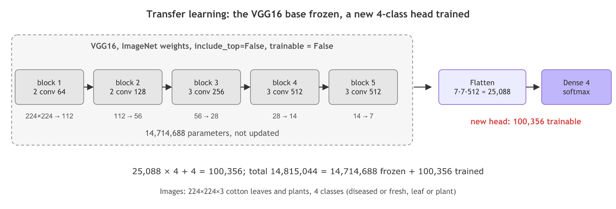
The summary shows the ideas of this part at full scale. Each 3×3 convolution with same padding keeps the size (224 + 2 − 3 + 1 = 224), and each 2×2 pool halves it: 224 → 112 → 56 → 28 → 14 → 7. block1_conv1 has 3·3·3·64 + 64 = 1,792 parameters and block1_conv2 3·3·64·64 + 64 = 36,928. The flattened 7×7×512 = 25,088 values feed Dense(4): 25,088·4 + 4 = 100,356 trainable parameters, against 14,714,688 frozen ones.
Augmenting the training images
ImageDataGenerator rescales the pixels to 0-1 and, for the training images only, applies random changes each time an image is used: a shear of up to 0.2 degrees (shear_range is an angle), a zoom of up to 20% and a horizontal flip. The network sees a slightly different leaf every epoch, which works like more data and reduces overfitting. The test images are only rescaled.
# Use the Image Data Generator to import the images from the dataset
from tensorflow.keras.preprocessing.image import ImageDataGenerator

train_datagen = ImageDataGenerator(rescale = 1./255,
                                   shear_range = 0.2,
                                   zoom_range = 0.2,
                                   horizontal_flip = True)

test_datagen = ImageDataGenerator(rescale = 1./255)# Make sure you provide the same target size as initialied for the image size
training_set = train_datagen.flow_from_directory('Datasets/train',
target_size = (224, 224),
batch_size = 32,
class_mode = 'categorical')Found 1951 images belonging to 4 classes.
test_set = test_datagen.flow_from_directory('Datasets/test',
                                            target_size = (224, 224),
                                            batch_size = 32,
class_mode = 'categorical')Found 18 images belonging to 4 classes.
Training the new head
Compiling uses categorical cross-entropy, because class_mode='categorical' gives one-hot labels (Categorical cross-entropy), and Adam. fit_generator trains for 20 epochs of 61 steps: 1,951 images in batches of 32.
# tell the model what cost and optimization method to use
model.compile(
  loss='categorical_crossentropy',
  optimizer='adam',
  metrics=['accuracy']
)# fit the model
# Run the cell. It will take some time to execute
r = model.fit_generator(
training_set,
validation_data=test_set,
epochs=20,
steps_per_epoch=len(training_set),
validation_steps=len(test_set)
)WARNING:tensorflow:From <ipython-input-16-2d02736eff38>:8: Model.fit_generator (from tensorflow.python.keras.engine.training) is deprecated and will be removed in a future version. Instructions for updating: Please use Model.fit, which supports generators. Epoch 1/20 61/61 [==============================] - 26s 431ms/step - loss: 3.0535 - accuracy: 0.3829 - val_loss: 1.4002 - val_accuracy: 0.3333 Epoch 2/20 61/61 [==============================] - 19s 316ms/step - loss: 1.0344 - accuracy: 0.5889 - val_loss: 1.0645 - val_accuracy: 0.6111 Epoch 3/20 61/61 [==============================] - 19s 312ms/step - loss: 0.9701 - accuracy: 0.6130 - val_loss: 1.6296 - val_accuracy: 0.5556 ... Epoch 15/20 61/61 [==============================] - 19s 313ms/step - loss: 0.6037 - accuracy: 0.7658 - val_loss: 0.7324 - val_accuracy: 0.7222 Epoch 16/20 61/61 [==============================] - 19s 313ms/step - loss: 0.6356 - accuracy: 0.7442 - val_loss: 0.5265 - val_accuracy: 0.8333 Epoch 17/20 61/61 [==============================] - 19s 313ms/step - loss: 0.7198 - accuracy: 0.7201 - val_loss: 0.6063 - val_accuracy: 0.7778 Epoch 18/20 61/61 [==============================] - 19s 314ms/step - loss: 0.7286 - accuracy: 0.7253 - val_loss: 1.2033 - val_accuracy: 0.6667 Epoch 19/20 61/61 [==============================] - 19s 312ms/step - loss: 0.7342 - accuracy: 0.7283 - val_loss: 1.7967 - val_accuracy: 0.5000 Epoch 20/20 61/61 [==============================] - 19s 313ms/step - loss: 0.9277 - accuracy: 0.6914 - val_loss: 0.6113 - val_accuracy: 0.7778
Training accuracy climbs from 0.38 to about 0.72 to 0.77. Validation accuracy jumps between 0.50 and 0.83 from one epoch to the next because the test folder holds only 18 images: one image more or less is 5.6 percentage points. The last epoch ends at 0.6914 training and 0.7778 validation accuracy. Its first line is TensorFlow 2.2's warning that fit_generator is deprecated in favour of fit.
Reading the notebook's stale cells
The notebook's later cells save the model and predict the 18 test images (the argmax gives one class index per image, such as 3, 2, 0). After that, several cells were copied from another project and do not belong to this model:
- Loading the wrong file: a cell loads
model_resnet50.h5, while the notebook savedmodel_vgg16.h5. - A variable shown before it exists:
img_datais printed before the cell that creates it. - Another dataset's path: the test image is read from
Datasets/Test/Coffee/, not from the cotton folders. - Preprocessing twice:
preprocess_inputis never imported and is applied afterx/255; VGG16's own preprocessing expects pixels from 0 to 255. - Two outputs from a 4-class model: the prediction prints
[[0.9745471, 0.0254529]], which only a 2-class model gives. - Blank plot files:
plt.savefigruns afterplt.show(), which has already cleared the figure.
Updating the notebook for Keras 3
TensorFlow 2.16 and later ship Keras 3, where several of the notebook's calls are gone or deprecated: fit_generator is removed (use fit), ImageDataGenerator is replaced by image_dataset_from_directory plus augmentation layers, the tf.compat.v1 session for GPU memory is not needed (tf.config.experimental.set_memory_growth does that), and models save as .keras rather than .h5.
Data and the frozen base
import keras
from keras import layers
from keras.applications import VGG16
from keras.applications.vgg16 import preprocess_input

train = keras.utils.image_dataset_from_directory("Datasets/train", image_size=(224, 224),
                                                 batch_size=32, label_mode="categorical")
test = keras.utils.image_dataset_from_directory("Datasets/test", image_size=(224, 224),
                                                batch_size=32, label_mode="categorical")
base = VGG16(weights="imagenet", include_top=False, input_shape=(224, 224, 3))
base.trainable = False                                   # freeze the whole base
Augmentation layers and the head
inputs = keras.Input(shape=(224, 224, 3))
x = layers.RandomFlip("horizontal")(inputs)             # horizontal_flip=True
x = layers.RandomZoom(0.2)(x)                             # zoom_range=0.2
x = layers.RandomShear(x_factor=0.2)(x)                   # shears up to 20% of the width
x = base(preprocess_input(x), training=False)            # VGG16's own scaling of 0-255 pixels
outputs = layers.Dense(4, activation="softmax")(layers.Flatten()(x))
model = keras.Model(inputs, outputs)
model.compile(optimizer="adam", loss="categorical_crossentropy", metrics=["accuracy"])
model.fit(train, validation_data=test, epochs=20)
model.save("model_vgg16.keras")
The augmentation layers are active only during training, and preprocess_input replaces the 1/255 rescale with the scaling VGG16 was trained on. RandomShear measures the shear as a fraction of the image width, not as an angle, so 0.2 here shears far more than the notebook's 0.2 degrees; lower it for a gentler shear. This version is shown, not run: it needs TensorFlow and the cotton dataset.
Counting VGG16's parameters
The summary's numbers come from the formulas of this part. The program also counts the ImageNet top that include_top=False dropped, and shows the horizontal flip on a tiny array.
import numpy as np

blocks = [(64, 2), (128, 2), (256, 3), (512, 3), (512, 3)]    # (filters, conv layers) per VGG16 block
size, c_in, base = 224, 3, 0
for b, (k, convs) in enumerate(blocks, 1):
    for _ in range(convs):
        base += 3 * 3 * c_in * k + k                            # f*f*C*k + k; 'same' padding keeps the size
        c_in = k
    size //= 2                                                  # 2x2 max pool, stride 2
    print(f"block {b}: {size}x{size}x{k}")
flat = size * size * c_in
head = flat * 4 + 4                                             # Dense(4) on the flattened output
print("frozen base:", base, " flatten:", flat, " new head:", head, " total:", base + head)
top = (flat * 4096 + 4096) + (4096 * 4096 + 4096) + (4096 * 1000 + 1000)
print("the dropped ImageNet top:", top, " full VGG16:", base + top)

leaf = np.arange(9).reshape(3, 3)                               # a tiny 3x3 'image'
print("horizontal flip:")
print(np.fliplr(leaf))block 1: 112x112x64 block 2: 56x56x128 block 3: 28x28x256 block 4: 14x14x512 block 5: 7x7x512 frozen base: 14714688 flatten: 25088 new head: 100356 total: 14815044 the dropped ImageNet top: 123642856 full VGG16: 138357544 horizontal flip: [[2 1 0] [5 4 3] [8 7 6]]
What the counts show
- The five blocks end at 112, 56, 28, 14 and 7 pixels, with 64 up to 512 channels, as in the saved summary.
- The frozen base has 14,714,688 parameters and the new head 100,356; the total, 14,815,044, matches the summary's Total params.
- The dropped ImageNet top has 123,642,856 parameters, so the full VGG16 has 138,357,544: almost 90% of it sits in the three dense layers.
- A horizontal flip reverses each row, 0 1 2 becoming 2 1 0, which is what
horizontal_flip=Truedoes to a photo.
Transfer learning vs training from scratch
| From scratch (CIFAR-10 CNN) | Transfer learning (VGG16) | |
|---|---|---|
| Filters | learned from random values | taken from ImageNet, frozen |
| Trainable parameters | 122,570, all of them | 100,356 of 14,815,044 |
| Training images | 50,000 | 1,951 |
| Input size | 32×32×3 | 224×224×3 |
| Training cost | every layer, every step | only the head; the base runs forward only |
Where you use transfer learning
- Small image datasets such as plant disease, medical scans or factory defects, where a few thousand labelled photos are all there is.
- Fast baselines: a frozen base and a new head train in minutes and often beat a model trained from scratch.
- Fine-tuning: after the head has trained, unfreeze the last block with a small learning rate to adapt the deepest filters to the new images.
preprocess_input as well; the model then sees inputs unlike anything it trained on, and its predictions are wrong with no error message.Related
- Previous: CNN in Keras
- Next: Neural network from scratch in NumPy
- Reference: Keras guide: Transfer learning and fine-tuning
- Reference: VGG16 in the Keras applications API
- Change the 4 in
head = flat * 4 + 4to the number of classes of your own dataset and read the new head size. - Replace the last pool's 7×7 flatten with global average pooling (512 values) and recompute the head: 512·4 + 4.
- Flip
leafvertically withnp.flipudand think about whether an upside-down cotton leaf is still a fair training image.
This is what real progress feels like.