Preparing the churn data
Preparing the churn data is the feature engineering step that turns the bank's Churn_Modelling.csv into numbers an ANN can learn from: choosing the columns, one-hot encoding Geography and Gender, splitting into train and test sets and standard scaling.
Last updated: 05 Oct, 2026 · pandas 3 · scikit-learn 1.9.1
The theory lessons, from Perceptron to Dropout, come together in one practical: a network that predicts whether a bank customer will leave. Before any Keras code, the data has to be cleaned and scaled with pandas and scikit-learn.
The video works in Google Colab with a GPU runtime and starts with !pip install tensorflow-gpu, which installs TensorFlow 2.8.0. That package has been discontinued: plain tensorflow includes GPU support, and Colab has it installed already. Installing TensorFlow covers a local install.
Loading Churn_Modelling.csv
The video imports NumPy, Matplotlib and pandas, with a comment on every cell, and reads Churn_Modelling.csv. Each row is a bank customer: a row number, a customer id, a surname, a credit score, a country (Geography), a gender, an age, a tenure, a balance, the number of products, whether they hold a credit card, whether they are an active member, an estimated salary and Exited, 1 if the customer left the bank. Predicting Exited is a binary classification problem; if the bank knows who is likely to leave, it can offer them more services. Exited is the dependent feature and the rest are independent features.
RowNumber is a running number, CustomerId is a unique value and a Surname does not decide whether someone leaves, so the independent features start at index 3 (CreditScore) and stop before index 13. dataset.iloc[:,3:13] takes all rows and columns 3 to 12; dataset.iloc[:,13] takes column 13, Exited.
The video drags the CSV into Colab's file pane. The same file is in the 2024 ANN-CLassification-Churn repository, so the code here reads it from GitHub by its raw URL and nothing has to be downloaded.
dataset=pd.read_csv(url)      # 10,000 customers
X=dataset.iloc[:,3:13]        # CreditScore ... EstimatedSalary
y=dataset.iloc[:,13] # Exited: 1 = left the bankimport pandas as pd
url = "https://raw.githubusercontent.com/krishnaik06/ANN-CLassification-Churn/main/Churn_Modelling.csv"
dataset=pd.read_csv(url)
X=dataset.iloc[:,3:13]
y=dataset.iloc[:,13]
pd.set_option("display.width", 200, "display.max_columns", 20) # all columns on one line
print(dataset.shape)
print(X.head())
print(y.value_counts())(10000, 14) CreditScore Geography Gender Age Tenure Balance NumOfProducts HasCrCard IsActiveMember EstimatedSalary 0 619 France Female 42 2 0.00 1 1 1 101348.88 1 608 Spain Female 41 1 83807.86 1 0 1 112542.58 2 502 France Female 42 8 159660.80 3 1 0 113931.57 3 699 France Female 39 1 0.00 2 0 0 93826.63 4 850 Spain Female 43 2 125510.82 1 1 1 79084.10 Exited 0 7963 1 2037 Name: count, dtype: int64
- 10,000 rows and 14 columns, of which X keeps 10: CreditScore to EstimatedSalary.
- The first rows match the video's
X.head(): 619, France, Female, 42, 2, 0.00, 1, 1, 1, 101348.88 for the first customer. - 7,963 customers stayed and 2,037 left, about 20% churn. A model that always says "stays" is already right about 80% of the time, which matters when reading the accuracy later.
Encoding Geography and Gender with get_dummies
Two of the independent features are categories, Geography and Gender, and a network multiplies numbers by weights, so they must become numbers. Both have very few categories, so one-hot encoding fits; pandas does it with pd.get_dummies. For Geography it makes one column per country, France, Germany and Spain, with a 1 in the column of that row's country and 0 elsewhere.
drop_first=True drops the first column. Two columns, Germany and Spain, still say everything: if both are 0, the customer is from France. Gender becomes a single column, Male. The video stores the results as geography and gender.
geography=pd.get_dummies(X['Geography'],drop_first=True)
gender=pd.get_dummies(X['Gender'],drop_first=True)print(pd.get_dummies(X['Geography']).head())
print(pd.get_dummies(X['Geography'],drop_first=True).head())
print(pd.get_dummies(X['Gender'],drop_first=True,dtype=int).head(3))France Germany Spain 0 True False False 1 False False True 2 True False False 3 True False False 4 False False True Germany Spain 0 False False 1 False True 2 False False 3 False False 4 False True Male 0 0 1 0 2 0
The video's pandas printed these columns as 1 and 0. Since pandas 2.0, get_dummies returns True and False (a bool column) unless you pass dtype=int, as in the last print. Scikit-learn and Keras treat True and False as 1 and 0, so the rest of the code works either way.
Dropping, joining and splitting the columns
The original Geography and Gender columns are no longer needed, so the video drops them with axis=1 (columns, not rows) and joins the new dummy columns with pd.concat(..., axis=1). It runs each line once without the X= first, to see that the result is right before replacing X. The result has 11 columns: the 8 numeric ones plus Germany, Spain and Male.
X=X.drop(['Geography','Gender'],axis=1)
X=pd.concat([X,geography,gender],axis=1)
Then Train and test split keeps 20% of the customers aside as the test set, with random_state=0 so the split repeats.
from sklearn.model_selection import train_test_split
X_train,X_test,y_train,y_test=train_test_split(X,y,test_size=0.2,random_state=0)Deciding which algorithms need feature scaling
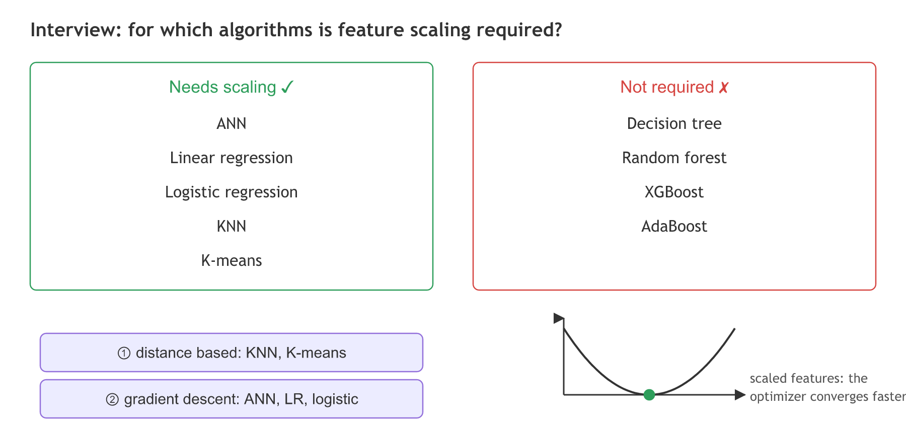
Before scaling, the video asks an interview question: for which algorithms is feature scaling required? There are two reasons to scale. Distance-based algorithms such as K nearest neighbours (KNN) and K-means clustering compare distances, and a feature with large values (a balance of 125,510) would swamp one with small values (a tenure of 2). Algorithms trained by gradient descent or another optimizer, the ANN, linear regression and logistic regression, converge much faster when the features are on similar scales. Tree-based models, a decision tree, random forest, XGBoost and AdaBoost, split one feature at a time on a threshold, so scaling does not change them.
Scaling the features with StandardScaler
StandardScaler turns every column into a z-score: it subtracts the column's mean and divides by its standard deviation, so each feature ends up centred on 0 with a standard deviation of 1.
The scaler is fitted on the training set only: fit_transform learns μ and σ from X_train and scales it, and transform applies the same μ and σ to X_test. Fitting on the test set as well would let information about the test data leak into training, the data leakage answer to the second interview question in the clip.
The video adds that MinMaxScaler, which squeezes values into 0 to 1, is for CNNs. Image pixels are scaled to 0 to 1, but the CNN practical does it by dividing by 255; either scaler can be used on tabular data.
from sklearn.preprocessing import StandardScaler
sc=StandardScaler()
X_train=sc.fit_transform(X_train)
X_test=sc.transform(X_test)
Running the whole preparation
import pandas as pd

url = "https://raw.githubusercontent.com/krishnaik06/ANN-CLassification-Churn/main/Churn_Modelling.csv"
dataset=pd.read_csv(url)
X=dataset.iloc[:,3:13]
y=dataset.iloc[:,13]
geography=pd.get_dummies(X['Geography'],drop_first=True)
gender=pd.get_dummies(X['Gender'],drop_first=True)
X=X.drop(['Geography','Gender'],axis=1)
X=pd.concat([X,geography,gender],axis=1)
from sklearn.model_selection import train_test_split
X_train,X_test,y_train,y_test=train_test_split(X,y,test_size=0.2,random_state=0)
from sklearn.preprocessing import StandardScaler
sc=StandardScaler()
X_train=sc.fit_transform(X_train)
X_test=sc.transform(X_test)

print(list(X.columns))
print(X_train)
print(X_train.shape, X_test.shape)
print("mean of CreditScore and Age in train:", sc.mean_[:2].round(2))
print("std of CreditScore and Age in train: ", sc.scale_[:2].round(2))['CreditScore', 'Age', 'Tenure', 'Balance', 'NumOfProducts', 'HasCrCard', 'IsActiveMember', 'EstimatedSalary', 'Germany', 'Spain', 'Male'] [[ 0.16958176 -0.46460796 0.00666099 ... -0.5698444 1.74309049 -1.09168714] [-2.30455945 0.30102557 -1.37744033 ... 1.75486502 -0.57369368 0.91601335] [-1.19119591 -0.94312892 -1.031415 ... -0.5698444 -0.57369368 -1.09168714] ... [ 0.9015152 -0.36890377 0.00666099 ... -0.5698444 -0.57369368 0.91601335] [-0.62420521 -0.08179119 1.39076231 ... -0.5698444 1.74309049 -1.09168714] [-0.28401079 0.87525072 -1.37744033 ... 1.75486502 -0.57369368 -1.09168714]] (8000, 11) (2000, 11) mean of CreditScore and Age in train: [650.55 38.85] std of CreditScore and Age in train: [97. 10.45]
What the scaled training set shows
- 11 columns: CreditScore, Age, Tenure, Balance, NumOfProducts, HasCrCard, IsActiveMember, EstimatedSalary, Germany, Spain and Male.
- The scaled X_train is the video's, number for number: the first row starts 0.16958176, −0.46460796, 0.00666099 and ends −1.09168714. The split and the scaler are deterministic, so the same rows come out every time.
- 8,000 training rows and 2,000 test rows, each with 11 features: the 11 inputs of the network in Building an ANN in Keras.
- CreditScore had a mean of 650.55 and a standard deviation of 97.0 in the training set, so a score of 667 becomes (667 − 650.55)/97 = 0.17, the first value of the first row.
- The video's run printed a UserWarning ("X has feature names, but StandardScaler was fitted without feature names"). It came from running the cell a second time after X_train had already become a NumPy array; a clean run in order gives no warning.
StandardScaler vs MinMaxScaler
| StandardScaler | MinMaxScaler | |
|---|---|---|
| Formula | (x − mean) / std | (x − min) / (max − min) |
| Result | mean 0, std 1, no fixed range | every value in [0, 1] |
| Outliers | stretch the std but stay visible | squeeze all other values together |
| Typical use | tabular data for ANNs, linear and logistic models | bounded data such as pixels |
Where you use this preparation
- Any tabular ANN: identifier columns out, categories one-hot encoded, a split, then a scaler fitted on the training data.
- Comparing an ANN with machine learning models on the same data: the video notes that this problem can also be solved with machine learning, and the prepared X_train feeds a logistic regression or a random forest unchanged.
- Serving a model: the 2024 version of this practical pickles the encoders and the scaler so new customers are prepared with the training set's numbers.
sc.fit_transform(X_test) instead of sc.transform(X_test) raises no error and still gives scaled numbers, but they use the test set's own mean and standard deviation. The test score then no longer measures how the model does on unseen data.Related
- Previous: Dropout
- Next: Building an ANN in Keras
- See also: Train and test split, Logistic regression
- Reference: StandardScaler in the scikit-learn API
- Remove
drop_first=Truefrom bothget_dummiescalls and check that X now has 14 columns. - Print
X_test.mean(axis=0).round(2): the test columns are close to 0 but not exactly 0, because the scaler was fitted on the training set. - Change
test_size=0.2to0.25and read the newX_train.shape.
Slow is fine. Stopping is the only problem.