CNN architecture
A CNN architecture is the order of layers in a convolutional network: convolution and pooling blocks that extract features, a flatten layer, and fully connected layers that end in one output per class.
Last updated: 05 Oct, 2026 · NumPy
Max pooling ended with small pooled maps. This lesson connects them to a classifier and traces the shapes through a whole network.
Flattening the pooled maps
Each filter gives its own pooled map: the cat-eye filter gives 5 7 / 3 5, another filter 7 9 / 2 1, another 6 5 / 3 1. Convolution and max pooling form one block, and the block can be stacked any number of times.
Then comes the flattening layer. It takes every pooled map and elongates it into one long column, the way an ANN takes its inputs: 5 7 3 5, then 7 9 2 1 attached below, then 6 5 3 1. That column is the input of a fully connected (dense) layer with ReLU, which ends in the outputs, here cat and dog.
The whole pipeline is: convolution (with padding and filters), max pooling, flattening, an ANN of fully connected layers, and the output.
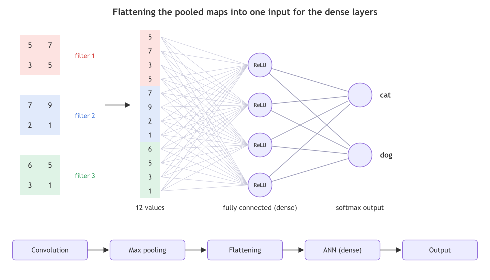
The board joins whole maps one after another. Keras' Flatten reads the array in (row, column, channel) order, so it interleaves the maps: 5 7 6, then 7 9 5, and so on. The dense layer learns a weight for each position, so either order works as long as it is the same every time.
Ending with softmax
The course notes' complete example ends with a softmax layer that turns the scores into probabilities, for example horse 0.2, zebra 0.7 and dog 0.1. The conv and pool blocks are the feature extraction part and the flatten, dense and softmax layers the classification part. The loss compares the probabilities with the true class (Softmax, Categorical cross-entropy).
Tracing the shapes of the MNIST CNN
The notes annotate a CNN for MNIST digits (28×28 grayscale, classes 0 to 9). A 5×5 convolution without padding gives 28 − 5 + 1 = 24, a 2×2 max pool 12, another 5×5 convolution 12 − 5 + 1 = 8, another pool 4. The 4×4 maps are flattened, go through two fully connected layers (the second with dropout, see Dropout) and end in 10 outputs.
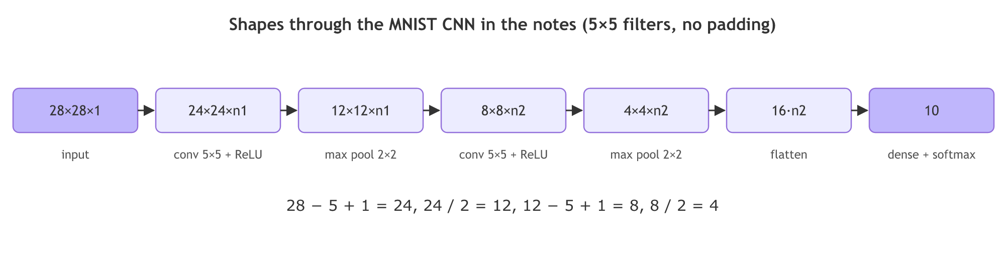
Running the board's numbers through the dense layers
Flattening the maps
reshape(-1) joins the maps one after another, as the board does. Moving the map axis to the end first gives the Keras order.
maps = np.array([[[5, 7], [3, 5]], [[7, 9], [2, 1]], [[6, 5], [3, 1]]])
x = maps.reshape(-1)                          # board order: 12 values
keras_order = maps.transpose(1, 2, 0).reshape(-1)
The dense layer and softmax
h = np.maximum(0, x @ W1 + b1)                # 12 inputs -> 4 ReLU neurons
z = h @ W2 + b2                               # 4 -> 2 scores: cat, dog
p = np.exp(z) / np.exp(z).sum()               # softmax
A forward pass from pooled maps to cat and dog
The weights are random, as before training, so the probabilities say nothing yet about cats; the shapes and the flow are the point.
import numpy as np

maps = np.array([[[5, 7], [3, 5]], [[7, 9], [2, 1]], [[6, 5], [3, 1]]])   # 3 pooled 2x2 maps
x = maps.reshape(-1)                                  # flatten map by map, as on the board
print("flattened:", x, " length", x.size)
print("Keras order (height, width, channels):", maps.transpose(1, 2, 0).reshape(-1))

rng = np.random.default_rng(42)
W1, b1 = rng.normal(0, 0.1, (12, 4)), np.zeros(4)     # dense layer: 12 inputs, 4 ReLU neurons
W2, b2 = rng.normal(0, 0.1, (4, 2)), np.zeros(2)      # output layer: cat, dog
h = np.maximum(0, x @ W1 + b1)
z = h @ W2 + b2
p = np.exp(z) / np.exp(z).sum()                       # softmax
print("hidden:", np.round(h, 3))
print("P(cat), P(dog):", np.round(p, 3), " sum", round(p.sum(), 3))
print("dense parameters:", W1.size + b1.size + W2.size + b2.size)

size, n2 = 28, 16                                     # MNIST, with 16 filters in the second conv as an example
for step, f in [("conv 5x5", 5), ("pool 2x2", 2), ("conv 5x5", 5), ("pool 2x2", 2)]:
    size = size - f + 1 if step.startswith("conv") else size // 2
    print(f"{step}: {size}x{size}")
print("flatten:", size * size * n2, "values")flattened: [5 7 3 5 7 9 2 1 6 5 3 1] length 12 Keras order (height, width, channels): [5 7 6 7 9 5 3 2 3 5 1 1] hidden: [0. 0. 2.843 1.006] P(cat), P(dog): [0.424 0.576] sum 1.0 dense parameters: 62 conv 5x5: 24x24 pool 2x2: 12x12 conv 5x5: 8x8 pool 2x2: 4x4 flatten: 256 values
What the forward pass shows
- The flattened vector has 12 values, 5 7 3 5 7 9 2 1 6 5 3 1, the board's column; Keras would order the same values as 5 7 6 7 9 5 3 2 3 5 1 1.
- The hidden layer holds four ReLU outputs; any neuron whose weighted sum is negative prints 0.
- The two probabilities are 0.424 and 0.576 and add up to 1: random weights give no real preference between cat and dog, only noise around 0.5.
- The dense part has 62 parameters: 12·4 + 4 for the hidden layer and 4·2 + 2 for the output.
- The MNIST trace prints 24, 12, 8 and 4, the notes' numbers, and 256 values after flattening with 16 filters.
Feature extraction vs classification
| Feature extraction | Classification | |
|---|---|---|
| Layers | Conv2D + ReLU, MaxPooling2D, repeated | Flatten, Dense + ReLU, Dense output |
| Input | the image grid | one long vector |
| Learns | filters: edges, textures, parts | which combinations of parts mean which class |
| Output | small maps with many channels | one score or probability per class |
| In transfer learning | reused from a trained network | replaced and trained for the new classes |
Where you use this architecture
- The CIFAR-10 model in CNN in Keras: three Conv2D layers, two pools, Flatten, Dense(64), Dense(10).
- VGG16 in Transfer learning with VGG16: five conv blocks, then Flatten and dense layers.
- Digit recognisers like the MNIST network in the notes, the classic first CNN.
Related
- Previous: Max pooling
- Next: CNN in Keras
- See also: Softmax
- Change
n2to 64 and see the flattened length grow to 1,024, the size of the CIFAR-10 model's Flatten layer. - Add a fourth pooled map
[[1, 2], [3, 4]], change W1's shape to (16, 4), and run the pass again. - Multiply
zby 10 before the softmax and watch the probabilities move away from 0.5.
You understood something today that you didn't yesterday.