CNN in Keras
A CNN in Keras is a Sequential model of Conv2D and MaxPooling2D layers followed by Flatten and Dense layers, trained with compile and fit like any other Keras model.
Last updated: 05 Oct, 2026 · TensorFlow 2 / Keras
Every layer from CNN architecture now becomes one line of code. The video runs TensorFlow's official tutorial “Convolutional Neural Network (CNN)” (cnn.ipynb) in Colab on the CIFAR-10 dataset and reads each cell. The outputs below are the ones on screen in that run (Colab, May 2022; the notebook does not print which TensorFlow 2 version it ran).
Loading and normalising CIFAR-10
CIFAR-10 has 60,000 colour images of 32×32 pixels in 10 classes (airplane, automobile, bird, cat, deer, dog, frog, horse, ship, truck), 6,000 per class: 50,000 for training and 10,000 for testing. The classes do not overlap. The first cell imports TensorFlow, Keras' datasets, layers and models, and matplotlib.
import tensorflow as tf

from tensorflow.keras import datasets, layers, models
import matplotlib.pyplot as plt
The second cell downloads the dataset and divides every pixel by 255.0, the normalising step from Convolution and filters.
(train_images, train_labels), (test_images, test_labels) = datasets.cifar10.load_data()

# Normalize pixel values to be between 0 and 1
train_images, test_images = train_images / 255.0, test_images / 255.0Downloading data from https://www.cs.toronto.edu/~kriz/cifar-10-python.tar.gz 170500096/170498071 [==============================] - 7s 0us/step 170508288/170498071 [==============================] - 7s 0us/step
The video says a pixel of 255 becomes 1 and the others 0. Dividing by 255.0 gives any value between 0 and 1: a pixel of 128 becomes 0.502.
The third cell plots the first 25 training images with their class names. On screen the first rows read frog, truck, truck, deer, automobile / automobile, bird, horse, ship, cat / deer, horse, horse, bird, truck / truck, truck, cat, bird, frog. The labels are arrays of one number each, hence train_labels[i][0].
class_names = ['airplane', 'automobile', 'bird', 'cat', 'deer',
               'dog', 'frog', 'horse', 'ship', 'truck']

plt.figure(figsize=(10,10))
for i in range(25):
    plt.subplot(5,5,i+1)
    plt.xticks([])
    plt.yticks([])
    plt.grid(False)
    plt.imshow(train_images[i])
    # The CIFAR labels happen to be arrays,
    # which is why you need the extra index
    plt.xlabel(class_names[train_labels[i][0]])
plt.show()
Building the convolutional base
As with the ANN, the model starts as models.Sequential(). Conv2D(32, (3, 3)) means 32 filters, each 3×3. ReLU follows the convolution. The input is an RGB image, 32×32 pixels with 3 channels, so input_shape=(32, 32, 3). Then come a 2×2 max pooling layer, a Conv2D with 64 filters, another pool, and a third Conv2D with 64 filters.
How many filters to use has no fixed rule: it is a hyperparameter. Try 32 or 64 and compare, or start from the numbers of well-known architectures.
model = models.Sequential()
model.add(layers.Conv2D(32, (3, 3), activation='relu', input_shape=(32, 32, 3)))
model.add(layers.MaxPooling2D((2, 2)))
model.add(layers.Conv2D(64, (3, 3), activation='relu'))
model.add(layers.MaxPooling2D((2, 2)))
model.add(layers.Conv2D(64, (3, 3), activation='relu'))model.summary()Model: "sequential" _________________________________________________________________ Layer (type) Output Shape Param # ================================================================= conv2d (Conv2D) (None, 30, 30, 32) 896 max_pooling2d (MaxPooling2D (None, 15, 15, 32) 0 ) conv2d_1 (Conv2D) (None, 13, 13, 64) 18496 max_pooling2d_1 (MaxPooling (None, 6, 6, 64) 0 2D) conv2d_2 (Conv2D) (None, 4, 4, 64) 36928 ================================================================= Total params: 56,320 Trainable params: 56,320 Non-trainable params: 0 _________________________________________________________________
The summary is the output-size formula at work. 32 − 3 + 1 = 30, pooling halves it to 15, 15 − 3 + 1 = 13, pooling gives ⌊13 / 2⌋ = 6, and 6 − 3 + 1 = 4. The parameter column counts the values inside the filters: (3·3·3 + 1)·32 = 896, (3·3·32 + 1)·64 = 18,496 and (3·3·64 + 1)·64 = 36,928. The video reads the first row as “an input of 30 cross 30”; 30×30×32 is that layer's output, and its input is 32×32×3.
In Keras 3 (TensorFlow 2.16 and later) passing input_shape to the first layer still runs but prints a warning; the current form starts the model with an Input layer:
model = models.Sequential([
    layers.Input(shape=(32, 32, 3)),
    layers.Conv2D(32, (3, 3), activation='relu'),
    layers.MaxPooling2D((2, 2)),
    # ... the same layers as above
])
Adding the dense layers
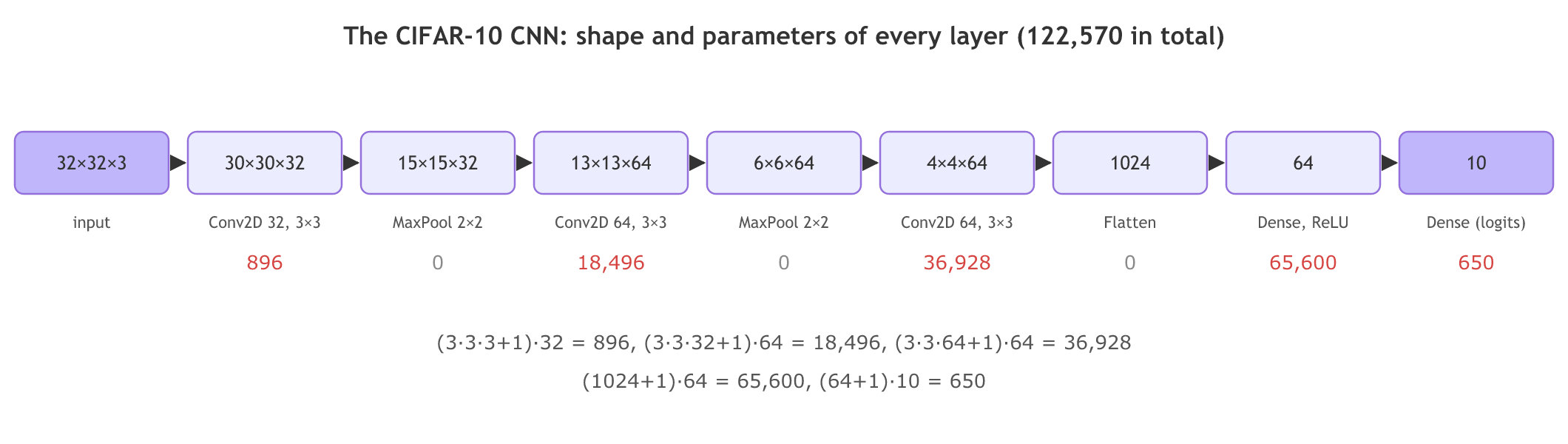
Flatten turns the 4×4×64 maps into 1,024 values. Dense(64, activation='relu') is the hidden layer and Dense(10) the output layer, one unit per class.
model.add(layers.Flatten())
model.add(layers.Dense(64, activation='relu'))
model.add(layers.Dense(10))model.summary()Model: "sequential" _________________________________________________________________ Layer (type) Output Shape Param # ================================================================= conv2d (Conv2D) (None, 30, 30, 32) 896 max_pooling2d (MaxPooling2D (None, 15, 15, 32) 0 ) conv2d_1 (Conv2D) (None, 13, 13, 64) 18496 max_pooling2d_1 (MaxPooling (None, 6, 6, 64) 0 2D) conv2d_2 (Conv2D) (None, 4, 4, 64) 36928 flatten (Flatten) (None, 1024) 0 dense (Dense) (None, 64) 65600 dense_1 (Dense) (None, 10) 650 ================================================================= Total params: 122,570 Trainable params: 122,570 Non-trainable params: 0 _________________________________________________________________
Flatten: 4·4·64 = 1,024. Dense(64): (1,024 + 1)·64 = 65,600. Dense(10): (64 + 1)·10 = 650. The total is 122,570. Dense(10) has no activation, so it outputs raw scores (logits), not probabilities.
Training and evaluating the model
The model is compiled with the Adam optimizer, the sparse categorical cross-entropy loss and accuracy as the metric, then trained for 10 epochs with the test images as validation data. The video picks the sparse loss “since we have 10 outputs”; the reason it is the sparse version is that the labels are integers 0 to 9 rather than one-hot vectors. from_logits=True is there because the last layer has no softmax: the loss applies it.
model.compile(optimizer='adam',
              loss=tf.keras.losses.SparseCategoricalCrossentropy(from_logits=True),
              metrics=['accuracy'])

history = model.fit(train_images, train_labels, epochs=10,
validation_data=(test_images, test_labels))Epoch 1/10 1563/1563 [==============================] - 23s 8ms/step - loss: 1.5322 - accuracy: 0.4408 - val_loss: 1.3039 - val_accuracy: 0.5342 Epoch 2/10 1563/1563 [==============================] - 12s 8ms/step - loss: 1.1702 - accuracy: 0.5846 - val_loss: 1.0451 - val_accuracy: 0.6300 Epoch 3/10 1563/1563 [==============================] - 12s 8ms/step - loss: 1.0151 - accuracy: 0.6405 - val_loss: 0.9910 - val_accuracy: 0.6570 Epoch 4/10 1563/1563 [==============================] - 13s 8ms/step - loss: 0.9095 - accuracy: 0.6813 - val_loss: 0.9402 - val_accuracy: 0.6749 Epoch 5/10 1563/1563 [==============================] - 12s 8ms/step - loss: 0.8338 - accuracy: 0.7090 - val_loss: 0.9055 - val_accuracy: 0.6844 Epoch 6/10 1563/1563 [==============================] - 13s 8ms/step - loss: 0.7761 - accuracy: 0.7264 - val_loss: 0.8560 - val_accuracy: 0.7029 Epoch 7/10 1563/1563 [==============================] - 12s 8ms/step - loss: 0.7250 - accuracy: 0.7454 - val_loss: 0.8684 - val_accuracy: 0.7008 Epoch 8/10 1563/1563 [==============================] - 13s 8ms/step - loss: 0.6848 - accuracy: 0.7597 - val_loss: 0.8350 - val_accuracy: 0.7138 Epoch 9/10 1563/1563 [==============================] - 12s 8ms/step - loss: 0.6430 - accuracy: 0.7752 - val_loss: 0.8472 - val_accuracy: 0.7137 Epoch 10/10 1563/1563 [==============================] - 13s 8ms/step - loss: 0.6098 - accuracy: 0.7860 - val_loss: 0.8851 - val_accuracy: 0.7040
The output box in the video is scrolled sideways, so the first six characters of every line are off screen: the epoch lines read “1/10” and the step lines “563 [====”. They are filled in above as Keras prints them, Epoch 1/10 and 1563/1563. The 1,563 total is on screen while epoch 1 runs (“1546/1563”), and every number after the cut-off is exactly as the frames show it.
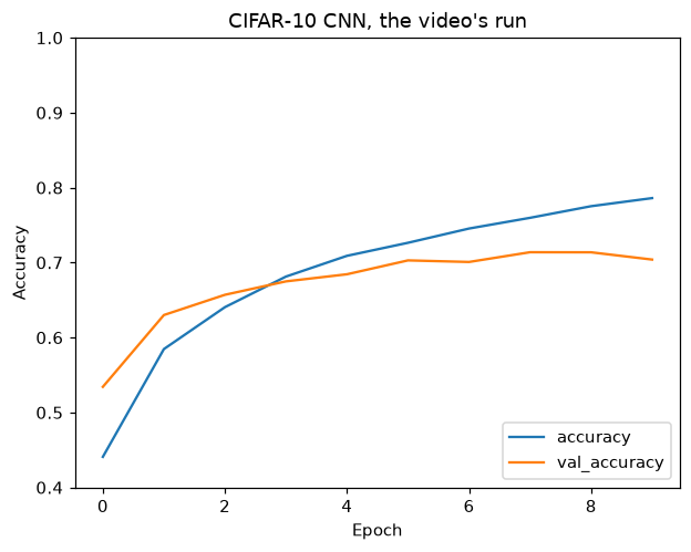
In epoch 1 validation accuracy (0.5342) is above training accuracy (0.4408). Training accuracy is averaged over the epoch while the weights are still improving, and validation accuracy is measured once at its end. The two lines cross between epochs 3 and 4 (between 2 and 3 on the plot, whose axis counts from 0), and from then on training accuracy pulls ahead.
The video says training was stopped when validation accuracy went down; all 10 epochs ran. Validation accuracy levels off near 0.70 to 0.71 from epoch 6 and dips to 0.7040 in epoch 10, while validation loss rises from 0.8350 in epoch 8 to 0.8851: the start of overfitting. Early stopping, which the video leaves as a task, would stop it there (Training and evaluating an ANN).
plt.plot(history.history['accuracy'], label='accuracy')
plt.plot(history.history['val_accuracy'], label = 'val_accuracy')
plt.xlabel('Epoch')
plt.ylabel('Accuracy')
plt.ylim([0.5, 1])
plt.legend(loc='lower right')

test_loss, test_acc = model.evaluate(test_images, test_labels, verbose=2)313/313 - 2s - loss: 0.8851 - accuracy: 0.7040 - 2s/epoch - 5ms/step
Under the evaluate line the cell draws the accuracy plot: training accuracy rises to about 0.79 and validation accuracy flattens near 0.70, with a widening gap after the lines cross. The video's advice is that this gap should be small.
print(test_acc)0.7039999961853027
The test accuracy is 0.704, so 70.4% (the video reads it as 70.3%). Ways to improve it from the video: more layers, more epochs and early stopping.
Plotting the run's accuracy curves
The training log gives every epoch's numbers, so the plot can be redrawn and the gap measured. These are the video's values, typed from the log above.
import matplotlib.pyplot as plt

# the video's run: epochs 1 to 10, from the training log
acc = [0.4408, 0.5846, 0.6405, 0.6813, 0.7090, 0.7264, 0.7454, 0.7597, 0.7752, 0.7860]
val_acc = [0.5342, 0.6300, 0.6570, 0.6749, 0.6844, 0.7029, 0.7008, 0.7138, 0.7137, 0.7040]
val_loss = [1.3039, 1.0451, 0.9910, 0.9402, 0.9055, 0.8560, 0.8684, 0.8350, 0.8472, 0.8851]

for e, (a, v) in enumerate(zip(acc, val_acc)):
    print(f"epoch {e + 1:2}: train {a:.4f}  val {v:.4f}  gap {a - v:+.4f}")
best = min(range(10), key=lambda i: val_loss[i])
print("lowest val_loss:", val_loss[best], "at epoch", best + 1)

plt.plot(acc, label="accuracy")
plt.plot(val_acc, label="val_accuracy")
plt.xlabel("Epoch")
plt.ylabel("Accuracy")
plt.ylim([0.4, 1])
plt.legend(loc="lower right")
plt.title("CIFAR-10 CNN, the video's run")
plt.show()epoch 1: train 0.4408 val 0.5342 gap -0.0934 epoch 2: train 0.5846 val 0.6300 gap -0.0454 epoch 3: train 0.6405 val 0.6570 gap -0.0165 epoch 4: train 0.6813 val 0.6749 gap +0.0064 epoch 5: train 0.7090 val 0.6844 gap +0.0246 epoch 6: train 0.7264 val 0.7029 gap +0.0235 epoch 7: train 0.7454 val 0.7008 gap +0.0446 epoch 8: train 0.7597 val 0.7138 gap +0.0459 epoch 9: train 0.7752 val 0.7137 gap +0.0615 epoch 10: train 0.7860 val 0.7040 gap +0.0820 lowest val_loss: 0.835 at epoch 8
Checking the summary's numbers
The shapes and parameter counts follow from two formulas, so NumPy-free Python reproduces the whole summary, and the 1,563 steps per epoch: 50,000 images in batches of 32 (the Keras default).
size, c_in, total = 32, 3, 0
for kind, k in [("conv", 32), ("pool", 0), ("conv", 64), ("pool", 0), ("conv", 64)]:
    if kind == "conv":
        params = (3 * 3 * c_in + 1) * k          # (f*f*C + 1) * k
        size, c_in = size - 3 + 1, k             # n - f + 1
    else:
        params, size = 0, size // 2              # 2x2 max pool
    total += params
    print(f"{kind}: {size}x{size}x{c_in}  params {params}")
flat = size * size * c_in
for units in (64, 10):
    params = (flat + 1) * units
    total += params
    print(f"dense {units}: params {params}")
    flat = units
print("total:", total)
print("steps per epoch:", -(-50000 // 32), " evaluate steps:", -(-10000 // 32))conv: 30x30x32 params 896 pool: 15x15x32 params 0 conv: 13x13x64 params 18496 pool: 6x6x64 params 0 conv: 4x4x64 params 36928 dense 64: params 65600 dense 10: params 650 total: 122570 steps per epoch: 1563 evaluate steps: 313
What the training log shows
- Every shape and count in the summary comes out of the two formulas: 30, 15, 13, 6, 4 and 122,570 parameters in total.
- 1,563 steps per epoch is 50,000 / 32 rounded up, and 313 evaluation steps is 10,000 / 32 rounded up.
- The gap starts negative (validation ahead) and grows to +0.082 by epoch 10.
- The lowest validation loss is 0.835, in epoch 8: early stopping on validation loss with patience 2 would stop at epoch 10 and keep epoch 8's weights if
restore_best_weights=True.
CNN vs ANN in Keras
| Churn ANN | CIFAR-10 CNN | |
|---|---|---|
| Input | 11 scaled features | 32×32×3 image, pixels / 255 |
| Layers | Dense only | Conv2D, MaxPooling2D, Flatten, Dense |
| Output layer | Dense(1, sigmoid) | Dense(10), logits |
| Loss | binary cross-entropy | sparse categorical cross-entropy, from_logits=True |
| Result | 85.9% test accuracy | 70.4% test accuracy after 10 epochs |
Where you use a Keras CNN
- A first model for any image dataset: a few Conv2D and pooling layers trained from scratch give a baseline in minutes on a Colab GPU.
- Small images such as CIFAR-10, digits, icons or product thumbnails, where a model of about 100,000 parameters is enough.
- A starting point for transfer learning, which swaps the convolutional base for a pretrained one (Transfer learning with VGG16).
from_logits must match the last layer. With Dense(10) and no activation, use from_logits=True. If you add activation='softmax' to the last layer, set from_logits=False; keeping True applies softmax twice, and training gets slower and less accurate without any error.Related
- Previous: CNN architecture
- Next: Transfer learning with VGG16
- Reference: TensorFlow tutorial: Convolutional Neural Network (CNN)
- Open the TensorFlow tutorial in Colab and add
keras.callbacks.EarlyStopping(monitor='val_loss', patience=2, restore_best_weights=True)tofit; compare the epoch it stops at with epoch 8 above. - In the summary check, change the first Conv2D to 16 filters and see which parameter counts change.
- Change
-(-50000 // 32)to use a batch size of 64 and predict the new step count before running.
Slow is fine. Stopping is the only problem.