How a neural network learns
A neural network learns by repeating a loop: a forward pass makes a prediction, a loss function measures how wrong it is, and backpropagation with an optimizer updates every weight so the next prediction is less wrong.
Last updated: 05 Oct, 2026 · NumPy
Forward propagation ended with predictions from weights that knew nothing. This lesson closes the loop: how the error flows back and changes the weights, and how many repeats of that turn a random network into a trained one.
Measuring the error with a loss function
Take the first record, 7, 3 and 7. It goes through the network and, with the weights initialised, say the output is 0. That 0 is the predicted value ŷ. The truth value y for this student is 1. Subtract them: y − ŷ = 1 − 0 = 1. That is not the output wanted, and the aim is to make this difference very near to zero.
The function that finds the difference between the predicted value and the real value is the loss function. There are different kinds, and the main aim is always to minimise it, so that ŷ and y match.
When the difference is large, the next step is back propagation. Its main aim is to update the weights: only by changing the weights can the predicted output come to match the real output, here 1 instead of 0. This is a supervised problem, with the right answer known for every training row, and the updating happens through back propagation.
Two notes on the clip. The output 0 is assumed for the story, not computed; the worked pass in Forward propagation gives a real ŷ of 0.511. And the raw difference y − ŷ can be negative, so it cannot be minimised as it stands (the board even writes it once as ŷ − y). Real loss functions square it, (y − ŷ)², or use cross-entropy, as Loss and cost functions explains.
Updating weights with an optimizer
The update itself is done by an optimizer, which makes sure every weight is updated while the error is propagated back. The video's example is gradient descent, the same idea as in simple linear regression: plot the loss against one weight and the curve is a U. From any starting point on the curve, the weight moves a small step downhill, and step after step it reaches the global minimum, where y − ŷ is smallest. The step is the slope times a learning rate η:
The clip calls gradient descent a combination of forward and backward propagation. More exactly, it is the update rule of the backward pass; each step needs a forward pass first to get ŷ and the loss.
How the slope ∂L/∂w is computed for every weight is the chain rule, the subject of Backpropagation and weight update and Chain rule of derivatives. The code below measures it a simpler way, by nudging each weight a little and watching the loss.
Repeating the loop until the network is trained
The whole story in seven steps. Forward propagation: (1) the input layer, (2) the weights, (3) the inputs times the weights added together with the bias, (4) the activation function, applied up to the last layer. Backward propagation: (5) the loss function, the difference between ŷ and y, (6) the optimizer, which minimises it by (7) updating the weights.
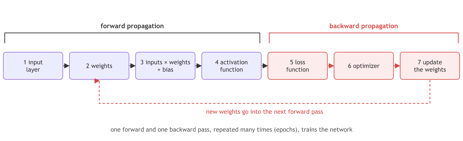
One forward pass and one backward pass, repeated a thousand times, train the network the way a baby is trained. Image classification, object detection, ANN, CNN and RNN all work on this forward and backward propagation, with different optimizers, and often far fewer repeats are enough. The video's example is a new flower: shown a black rose once, you may forget its name the next day; shown it day after day, you say "black rose" with confidence. Repetition is training.
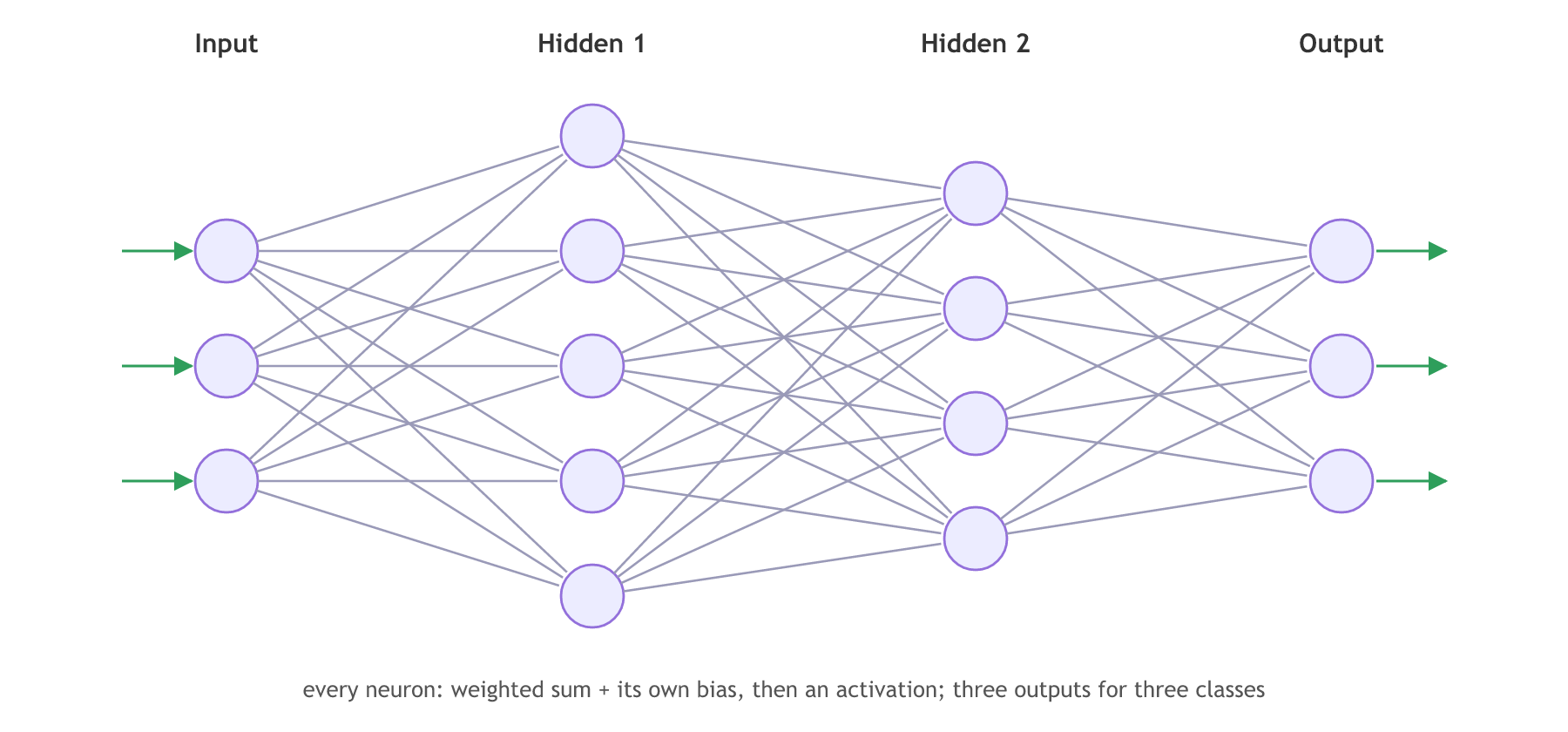
A multi-layer neural network follows the same process. It has many inputs, any number of hidden layers with any number of neurons, and for a multi-class problem several output neurons. Every layer adds its bias, every neuron does the same two steps. For multi-class problems only the activation function and the loss function change.
Training the notes' network in NumPy
The pieces below train the 3-1-1 network from the forward propagation lesson on its three students, starting from the notes' weights. The inputs are standard-scaled first, so IQ (around 95) and hours (2 to 7) sit on the same scale, as in Train and test split's scaling step.
The data, scaled
import numpy as np

X = np.array([[95, 4, 4], [100, 5, 2], [95, 2, 7]], dtype=float)   # IQ, study, play
y = np.array([1, 1, 0])
Xs = (X - X.mean(axis=0)) / X.std(axis=0)    # standard scaling, column by column
The forward pass and the loss
def predict(p, X):
    w, b1, w4, b2 = p[:3], p[3], p[4], p[5]
    o1 = 1 / (1 + np.exp(-(X @ w + b1)))         # hidden neuron
    return 1 / (1 + np.exp(-(o1 * w4 + b2)))      # output neuron

def loss(p, X):
    return np.mean((y - predict(p, X)) ** 2)      # mean squared error
The slope of the loss for each weight
def slopes(p, X, h=1e-6):
    # nudge each weight up and down a little and see how the loss changes
    return np.array([(loss(p + e, X) - loss(p - e, X)) / (2 * h) for e in np.eye(6) * h])
The training loop
def train(X, epochs=1000, lr=1.0):
    p = np.array([0.01, 0.02, 0.03, 0.001, 0.02, 0.03])   # the notes' starting weights
    for epoch in range(epochs + 1):
        if epoch % 250 == 0:
            print(f"epoch {epoch:4}  loss {loss(p, X):.4f}  predictions {np.round(predict(p, X), 3)}")
        p = p - lr * slopes(p, X)        # w_new = w_old - learning rate x slope
    return p
Running the training loop
p = train(Xs)
print("classes:", (predict(p, Xs) >= 0.5).astype(int), " true:", y)epoch 0 loss 0.2468 predictions [0.51 0.51 0.51] epoch 250 loss 0.0099 predictions [0.91 0.942 0.135] epoch 500 loss 0.0038 predictions [0.945 0.963 0.083] epoch 750 loss 0.0023 predictions [0.957 0.97 0.064] epoch 1000 loss 0.0016 predictions [0.964 0.975 0.054] classes: [1 1 0] true: [1 1 0]
Reading the training run
- Epoch 0 is the forward propagation lesson's result: every student near 0.51 and a loss of 0.2468.
- The loss falls with every repeat, fast at first and then slowly, the way gradient descent slows near the bottom of the U.
- The predictions separate: the two passing students climb towards 1, the failing one drops below 0.1, and the classes come out 1, 1, 0, matching the table.
- Nothing but the weights changed. The data, the network and the loss function stayed the same; the loop moved six numbers.
Loss function vs optimizer
| Loss function | Optimizer | |
|---|---|---|
| Job | Measures how wrong the predictions are | Changes the weights to make the loss smaller |
| Input | y and ŷ | The loss's slope for each weight |
| Output | One number | New weights |
| Examples | Squared error, binary and categorical cross-entropy | Gradient descent, SGD, Adam |
| Chosen by | The kind of problem (regression, binary, multi-class) | Speed and stability of training |
Where you use the training loop
- Keras
model.fitruns this loop: a forward pass on a batch, the loss, backpropagation, the optimizer step, repeated for the epochs you ask for. - Reading a training log: the falling loss per epoch that Keras prints is the column printed here.
- Interviews: "explain how a neural network is trained" is answered by the seven steps.
train(X): the IQ of about 95 swamps the hidden neuron's sum, so every student gets almost the same hidden output, which training then pushes into the flat end of the sigmoid. The loss gets stuck near 0.222 with every prediction about 0.667. The network can never tell the students apart. Scale the inputs first.Related
- Previous: Forward propagation
- Next: Backpropagation and weight update
- See also: Gradient descent in the Machine Learning course
- Run
train(X)on the unscaled table and compare its last line with the scaled run. - Change the learning rate to
lr=0.1and see how much higher the loss still is at epoch 1000. - Train for 3000 epochs and check how close the passing students get to 1.
You understood something today that you didn't yesterday.