Neural network from scratch in NumPy
A neural network from scratch is a fully connected network written with plain NumPy arrays, in which the weight initialization, the forward pass, the loss, backpropagation and the optimizer are each a few lines of code you can read and change.
Last updated: 05 Oct, 2026 · NumPy
The earlier lessons taught each piece on its own: weights and bias, the forward pass, the chain rule, activation functions, binary cross-entropy, weight initialization and the optimizers. Keras hides all of them behind fit(). Here they become one program that learns the two moons of scikit-learn's make_moons, and the same program then shows two ways training fails, with real output.
Following the network and its training loop
The network has 2 inputs, two hidden layers of 16 neurons and one sigmoid output neuron, written 2-16-16-1. Each neuron does the two steps from Weights and bias: a weighted sum plus a bias, then an activation. The loop is the seven steps of How a neural network learns: the inputs, weights, bias and activation make the forward pass; the loss, the optimizer and the weight update make the backward pass, repeated over many epochs.
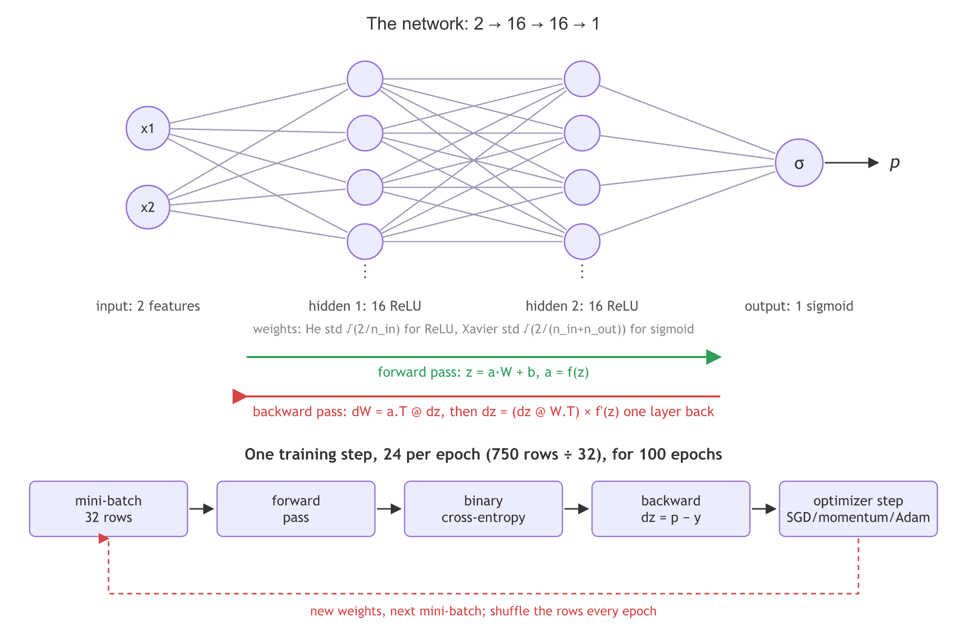
The training set has 750 rows. With mini-batches of 32 rows, one epoch is 24 weight updates (the last batch holds 14 rows), and the run lasts 100 epochs. SGD and mini-batch gradient descent explains the batch, iteration and epoch counts.
Loading make_moons and scaling it
make_moons draws two interleaving half circles of points, one per class. No straight line separates them, so a single neuron (logistic regression) cannot fit them and hidden layers are needed. noise=0.2 scatters the points so that the two moons overlap a little. The rows are split 750 / 250 with Train and test split, and the scaler learns its mean and spread from the training rows only. The labels become a column so that they line up with the network's output, which is one column of probabilities.
import numpy as np
from sklearn.datasets import make_moons
from sklearn.model_selection import train_test_split
from sklearn.preprocessing import StandardScaler

X, y = make_moons(n_samples=1000, noise=0.2, random_state=0)
X_train, X_test, y_train, y_test = train_test_split(X, y, test_size=0.25, random_state=0)
scaler = StandardScaler().fit(X_train)                    # learn the scale from the train rows only
X_train, X_test = scaler.transform(X_train), scaler.transform(X_test)
y_train, y_test = y_train.reshape(-1, 1), y_test.reshape(-1, 1)   # columns, to match the output
Writing the network in NumPy
Activation functions and their derivatives
Every activation needs its derivative for the backward pass. ReLU's derivative is 1 where z is positive and 0 elsewhere. The sigmoid's derivative is σ(z)(1 − σ(z)), which is at most 0.25, as Chain rule of derivatives showed. The dictionary ACT lets the same code switch between them by name.
def relu(z): return np.maximum(0, z)
def relu_grad(z): return (z > 0).astype(float)
def sigmoid(z): return 1 / (1 + np.exp(-z))
def sigmoid_grad(z): return sigmoid(z) * (1 - sigmoid(z))
ACT = {"relu": (relu, relu_grad), "sigmoid": (sigmoid, sigmoid_grad)}
Initializing the weights with He and Xavier
The weights start small, different from each other and with a variance that suits the activation, the three key points of Weight initialization. He normal, with a standard deviation of √(2 / n_in), goes with ReLU. Xavier (Glorot) normal, with √(2 / (n_in + n_out)), goes with sigmoid. Both formulas give a standard deviation, which is what rng.normal takes as its second argument. Biases start at 0, because the random weights already make the neurons different.
def init(sizes, act, seed=0):
    rng = np.random.default_rng(seed)
    params = []
    for n_in, n_out in zip(sizes[:-1], sizes[1:]):
        if act == "relu":
            std = np.sqrt(2 / n_in)               # He normal
        else:
            std = np.sqrt(2 / (n_in + n_out))     # Xavier (Glorot) normal
        params.append([rng.normal(0, std, (n_in, n_out)), np.zeros(n_out)])
    return params
The forward pass
Each layer computes z = a·W + b for every row at once, a matrix product, then applies the activation. The hidden layers use ReLU or sigmoid; the last layer always uses sigmoid, so its output p is a probability between 0 and 1. The list cache keeps each layer's input and z, because the backward pass needs both.
def forward(params, X, act):
    a, cache = X, []
    for i, (W, b) in enumerate(params):
        z = a @ W + b                          # step 1: weighted sum plus bias
        cache.append((a, z))                   # keep each layer's input and z for backprop
        last = i == len(params) - 1
        a = sigmoid(z) if last else ACT[act][0](z)   # step 2: activation
    return a, cache
Binary cross-entropy
The loss is the Binary cross-entropy averaged over the rows. np.clip keeps p a hair away from 0 and 1, so np.log never returns minus infinity. A network that outputs 0.5 for every row scores ln 2 = 0.693, the loss of a coin toss.
def bce(p, y):
    p = np.clip(p, 1e-12, 1 - 1e-12)           # keep log() away from 0
    return -np.mean(y * np.log(p) + (1 - y) * np.log(1 - p))
Backpropagation with the chain rule
Backpropagation starts at the output and walks back one layer at a time. With a sigmoid output and binary cross-entropy, the two derivatives ∂L/∂p and ∂p/∂z cancel into a short result: ∂L/∂z = p − y for each row. From there the chain rule gives every other gradient:
The last formula is one hop of the chain rule: multiply by the weights the signal came through, then by the activation's derivative. Each hop multiplies the gradient by another f′(z), which is where the vanishing gradient problem comes from. Dividing by the number of rows at the start makes the gradients those of the mean loss.
def backward(params, cache, p, y, act):
    grads = [None] * len(params)
    dz = (p - y) / len(y)                      # dL/dz at the output: sigmoid + BCE give p - y
    for i in reversed(range(len(params))):
        a_prev, _ = cache[i]
        grads[i] = [a_prev.T @ dz, dz.sum(axis=0)]     # dL/dW and dL/db of layer i
        if i > 0:
            z_prev = cache[i - 1][1]
            dz = (dz @ params[i][0].T) * ACT[act][1](z_prev)   # one hop back: times W, times f'(z)
    return grads
SGD, momentum and Adam by hand
All three use the weight update w = w − η × (a direction) from Backpropagation and weight update. Plain SGD steps along the gradient. Momentum steps along V, an exponentially weighted average of the gradients, V = βV + (1 − β)g, the form used in SGD with momentum. Adam keeps that average and also an average of the squared gradients S, divides one by the square root of the other, and corrects both for starting at zero, as in Adam optimizer. The v[:] = form writes into the stored arrays so they carry over to the next step.
def step(params, grads, state, kind, lr, t, b1=0.9, b2=0.999, eps=1e-8):
    for layer, g_layer, s_layer in zip(params, grads, state):
        for j, g in enumerate(g_layer):        # j = 0 the weights, j = 1 the bias
            v, s = s_layer[j]
            if kind == "sgd":
                layer[j] -= lr * g
            elif kind == "momentum":           # V = beta V + (1 - beta) g, as in the video
                v[:] = b1 * v + (1 - b1) * g
                layer[j] -= lr * v
            else:                              # adam: momentum + RMSprop + bias correction
                v[:] = b1 * v + (1 - b1) * g
                s[:] = b2 * s + (1 - b2) * g ** 2
                layer[j] -= lr * (v / (1 - b1 ** t)) / (np.sqrt(s / (1 - b2 ** t)) + eps)
Measuring loss and accuracy
After every epoch the program records two numbers: the loss on all 750 training rows and the accuracy on the 250 test rows, where a probability above 0.5 counts as class 1.
def evaluate(params, act):
    p_train, _ = forward(params, X_train, act)
    p_test, _ = forward(params, X_test, act)
    return bce(p_train, y_train), np.mean((p_test > 0.5) == y_test)
The mini-batch training loop
train builds the weights, an empty optimizer state for every weight and bias, and then runs the epochs. Each epoch shuffles the rows, cuts them into batches of 32, and for each batch runs the forward pass, the backward pass and one optimizer step. t counts the steps, for Adam's bias correction.
def train(sizes, act, kind, lr, epochs=100, batch=32, seed=0):
    params = init(sizes, act, seed)
    state = [[[np.zeros_like(q), np.zeros_like(q)] for q in layer] for layer in params]
    rng, t, history = np.random.default_rng(seed), 0, []
    for epoch in range(epochs):
        order = rng.permutation(len(X_train))          # shuffle the rows every epoch
        for start in range(0, len(order), batch):
            idx = order[start:start + batch]           # one mini-batch of 32 rows
            p, cache = forward(params, X_train[idx], act)
            t += 1
            step(params, backward(params, cache, p, y_train[idx], act), state, kind, lr, t)
        history.append(evaluate(params, act))          # (train loss, test accuracy)
    return params, history
Training a ReLU network on the moons end to end
The whole program, with a 2-16-16-1 ReLU network trained by Adam at a learning rate of 0.01:
import numpy as np
from sklearn.datasets import make_moons
from sklearn.model_selection import train_test_split
from sklearn.preprocessing import StandardScaler

X, y = make_moons(n_samples=1000, noise=0.2, random_state=0)
X_train, X_test, y_train, y_test = train_test_split(X, y, test_size=0.25, random_state=0)
scaler = StandardScaler().fit(X_train)                    # learn the scale from the train rows only
X_train, X_test = scaler.transform(X_train), scaler.transform(X_test)
y_train, y_test = y_train.reshape(-1, 1), y_test.reshape(-1, 1)   # columns, to match the output

def relu(z): return np.maximum(0, z)
def relu_grad(z): return (z > 0).astype(float)
def sigmoid(z): return 1 / (1 + np.exp(-z))
def sigmoid_grad(z): return sigmoid(z) * (1 - sigmoid(z))
ACT = {"relu": (relu, relu_grad), "sigmoid": (sigmoid, sigmoid_grad)}

def init(sizes, act, seed=0):
    rng = np.random.default_rng(seed)
    params = []
    for n_in, n_out in zip(sizes[:-1], sizes[1:]):
        if act == "relu":
            std = np.sqrt(2 / n_in)               # He normal
        else:
            std = np.sqrt(2 / (n_in + n_out))     # Xavier (Glorot) normal
        params.append([rng.normal(0, std, (n_in, n_out)), np.zeros(n_out)])
    return params

def forward(params, X, act):
    a, cache = X, []
    for i, (W, b) in enumerate(params):
        z = a @ W + b                          # step 1: weighted sum plus bias
        cache.append((a, z))                   # keep each layer's input and z for backprop
        last = i == len(params) - 1
        a = sigmoid(z) if last else ACT[act][0](z)   # step 2: activation
    return a, cache

def bce(p, y):
    p = np.clip(p, 1e-12, 1 - 1e-12)           # keep log() away from 0
    return -np.mean(y * np.log(p) + (1 - y) * np.log(1 - p))

def backward(params, cache, p, y, act):
    grads = [None] * len(params)
    dz = (p - y) / len(y)                      # dL/dz at the output: sigmoid + BCE give p - y
    for i in reversed(range(len(params))):
        a_prev, _ = cache[i]
        grads[i] = [a_prev.T @ dz, dz.sum(axis=0)]     # dL/dW and dL/db of layer i
        if i > 0:
            z_prev = cache[i - 1][1]
            dz = (dz @ params[i][0].T) * ACT[act][1](z_prev)   # one hop back: times W, times f'(z)
    return grads

def step(params, grads, state, kind, lr, t, b1=0.9, b2=0.999, eps=1e-8):
    for layer, g_layer, s_layer in zip(params, grads, state):
        for j, g in enumerate(g_layer):        # j = 0 the weights, j = 1 the bias
            v, s = s_layer[j]
            if kind == "sgd":
                layer[j] -= lr * g
            elif kind == "momentum":           # V = beta V + (1 - beta) g, as in the video
                v[:] = b1 * v + (1 - b1) * g
                layer[j] -= lr * v
            else:                              # adam: momentum + RMSprop + bias correction
                v[:] = b1 * v + (1 - b1) * g
                s[:] = b2 * s + (1 - b2) * g ** 2
                layer[j] -= lr * (v / (1 - b1 ** t)) / (np.sqrt(s / (1 - b2 ** t)) + eps)

def evaluate(params, act):
    p_train, _ = forward(params, X_train, act)
    p_test, _ = forward(params, X_test, act)
    return bce(p_train, y_train), np.mean((p_test > 0.5) == y_test)

def train(sizes, act, kind, lr, epochs=100, batch=32, seed=0):
    params = init(sizes, act, seed)
    state = [[[np.zeros_like(q), np.zeros_like(q)] for q in layer] for layer in params]
    rng, t, history = np.random.default_rng(seed), 0, []
    for epoch in range(epochs):
        order = rng.permutation(len(X_train))          # shuffle the rows every epoch
        for start in range(0, len(order), batch):
            idx = order[start:start + batch]           # one mini-batch of 32 rows
            p, cache = forward(params, X_train[idx], act)
            t += 1
            step(params, backward(params, cache, p, y_train[idx], act), state, kind, lr, t)
        history.append(evaluate(params, act))          # (train loss, test accuracy)
    return params, history

params, history = train([2, 16, 16, 1], "relu", "adam", lr=0.01)
for epoch in (1, 10, 50, 100):
    loss, acc = history[epoch - 1]
print(f"epoch {epoch:3} train loss {loss:.4f} test accuracy {acc:.3f}")epoch 1 train loss 0.2649 test accuracy 0.848 epoch 10 train loss 0.0971 test accuracy 0.968 epoch 50 train loss 0.0742 test accuracy 0.968 epoch 100 train loss 0.0736 test accuracy 0.964
What the training run shows
- The first epoch already lifts the test accuracy to 0.848, and the training loss is already 0.265, well below the 0.693 of a coin toss.
- By epoch 10 the network reaches 0.968 on the test rows. The loss keeps falling slowly after that, from 0.097 to 0.074, while the test accuracy stays near 0.96 to 0.97.
- The last few points do not improve because the moons overlap: with
noise=0.2, a few points sit on the wrong side of any sensible boundary.
Checking the chain rule with a numerical gradient
A bug in backpropagation does not crash: the network trains worse and nothing says why. The check is to nudge one weight by a small h, measure how the loss changes, and compare (L(w + h) − L(w − h)) / 2h with the gradient that backward returned for the same weight.
params = init([2, 16, 16, 1], "relu")
p, cache = forward(params, X_train, "relu")
grads = backward(params, cache, p, y_train, "relu")

W, h = params[0][0], 1e-5                     # nudge one weight up and down by h
W[0, 0] += h
loss_up = bce(forward(params, X_train, "relu")[0], y_train)
W[0, 0] -= 2 * h
loss_down = bce(forward(params, X_train, "relu")[0], y_train)
W[0, 0] += h                                  # put the weight back
print("backprop :", round(grads[0][0][0, 0], 8))
print("numerical:", round((loss_up - loss_down) / (2 * h), 8))backprop : 0.07794692 numerical: 0.07794692
The two numbers agree to about eight decimal places, so the chain rule in backward computes the true slope of the loss. Changing * ACT[act][1](z_prev) to * 1 in backward and running the check again makes the two numbers disagree.
Comparing sigmoid and ReLU hidden layers
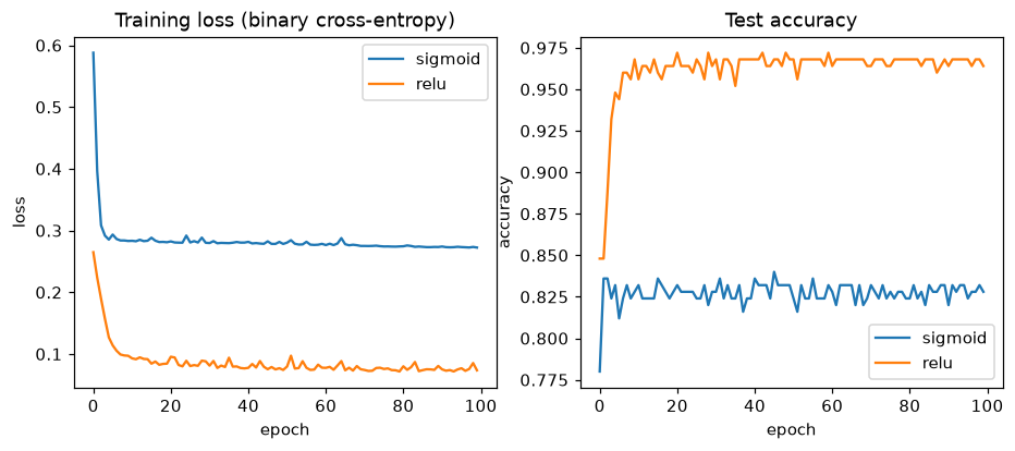
The same network, the same Adam optimizer and the same 100 epochs, with only the hidden activation changed. The sigmoid run uses Xavier initialization and the ReLU run He initialization, through init.
import matplotlib.pyplot as plt

runs = {act: train([2, 16, 16, 1], act, "adam", lr=0.01)[1] for act in ("sigmoid", "relu")}
fig, (ax1, ax2) = plt.subplots(1, 2, figsize=(10, 3.8))
for act, history in runs.items():
    loss, acc = zip(*history)
    ax1.plot(loss, label=act)
    ax2.plot(acc, label=act)
    print(f"{act:8} epoch 10: loss {loss[9]:.3f}  epoch 100: loss {loss[-1]:.3f}  test accuracy {acc[-1]:.3f}")
ax1.set(title="Training loss (binary cross-entropy)", xlabel="epoch", ylabel="loss")
ax2.set(title="Test accuracy", xlabel="epoch", ylabel="accuracy")
ax1.legend()
ax2.legend()
plt.show()sigmoid epoch 10: loss 0.283 epoch 100: loss 0.272 test accuracy 0.828 relu epoch 10: loss 0.097 epoch 100: loss 0.074 test accuracy 0.964
What the activation comparison shows
- ReLU ends at a test accuracy of 0.964 and a loss of 0.074.
- Sigmoid stops at 0.828 with a loss of 0.272. Its loss falls fast at first, then sits on a plateau: the network has learned a boundary close to a straight line, which gets about 83% of the moons right, and it bends that line very slowly.
- The difference is the derivative. σ′ is at most 0.25, so every hop back through a sigmoid layer shrinks the gradient, while ReLU passes it through unchanged wherever z is positive. ReLU and its variants covers the same point on the board.
Comparing SGD, momentum and Adam
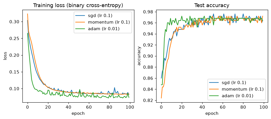
The ReLU network again, trained three ways. SGD and momentum use a learning rate of 0.1 and Adam 0.01, a common starting value for each. Keras's default for Adam is 0.001; 0.01 is set here so that 100 epochs are enough. Two numbers summarise each run: the first epoch at which the test accuracy reaches 0.95, and the wobble, the average change in the training loss from one epoch to the next after epoch 20.
import matplotlib.pyplot as plt

settings = {"sgd": 0.1, "momentum": 0.1, "adam": 0.01}      # optimizer: learning rate
fig, (ax1, ax2) = plt.subplots(1, 2, figsize=(10, 3.8))
for kind, lr in settings.items():
    loss, acc = map(np.array, zip(*train([2, 16, 16, 1], "relu", kind, lr)[1]))
    first = np.argmax(acc >= 0.95) + 1                        # first epoch at 95% test accuracy
    wobble = np.abs(np.diff(loss[20:])).mean()                # epoch-to-epoch change in the loss
    print(f"{kind:8} lr {lr:<4}  95% at epoch {first:2}  final loss {loss[-1]:.3f}  wobble {wobble:.4f}")
    ax1.plot(loss, label=f"{kind} (lr {lr})")
    ax2.plot(acc, label=f"{kind} (lr {lr})")
ax1.set(title="Training loss (binary cross-entropy)", xlabel="epoch", ylabel="loss")
ax2.set(title="Test accuracy", xlabel="epoch", ylabel="accuracy")
ax1.legend()
ax2.legend()
plt.show()sgd lr 0.1 95% at epoch 23 final loss 0.082 wobble 0.0029 momentum lr 0.1 95% at epoch 16 final loss 0.084 wobble 0.0007 adam lr 0.01 95% at epoch 7 final loss 0.074 wobble 0.0052
What the optimizer comparison shows
- Adam reaches 95% test accuracy first, at epoch 7, because it scales each weight's step by its own gradient history: weights with small gradients get relatively larger steps.
- Momentum gets there at epoch 16 and SGD at epoch 23. With V = βV + (1 − β)g the step is an average of recent gradients, so its size stays close to SGD's, but the noise of single batches cancels out.
- Momentum's wobble is about 4 times smaller than SGD's (0.0007 against 0.0029): the smoothing the video describes for the exponentially weighted average. Adam's wobble is the largest, because its larger relative steps keep moving the weights around the minimum.
- All three end close together, between 0.074 and 0.084 in loss. On a small problem the optimizer mostly changes how fast training gets there, not where it ends.
Making the early-layer gradients vanish
The first failure is the Vanishing gradient problem. The network grows to eight hidden layers of 16 neurons. The code runs one forward and backward pass on the training rows at initialization and prints the size of each layer's weight gradient, the first layer on the left and the output layer on the right, for sigmoid with Xavier and for ReLU with He. Then it trains the deep sigmoid network with SGD for 100 epochs.
deep = [2] + [16] * 8 + [1]                   # eight hidden layers of 16 neurons
for act in ("sigmoid", "relu"):
    params = init(deep, act)
    p, cache = forward(params, X_train, act)
    grads = backward(params, cache, p, y_train, act)
    norms = [np.linalg.norm(dW) for dW, db in grads]       # size of dL/dW, layer by layer
    print(f"{act:8}", " ".join(f"{n:.1e}" for n in norms))

_, history = train(deep, "sigmoid", "sgd", lr=0.1)
print("deep sigmoid after 100 epochs: loss", round(history[-1][0], 3), " test accuracy", history[-1][1])sigmoid 6.4e-06 2.5e-05 9.6e-05 4.7e-04 1.8e-03 6.3e-03 3.7e-02 1.3e-01 3.5e-01 relu 1.2e-01 2.1e-01 3.1e-01 3.4e-01 2.8e-01 3.3e-01 2.0e-01 3.4e-01 3.9e-01 deep sigmoid after 100 epochs: loss 0.694 test accuracy 0.532
Why the deep sigmoid network learned nothing
- The sigmoid gradients shrink 3 to 6 times per layer going back, from 3.5e-01 (0.35) at the output to 6.4e-06 at the first layer, about 55,000 times smaller. Each hop multiplies by σ′(z), at most 0.25, times weights of Xavier size.
- The ReLU gradients stay between about 0.1 and 0.4 in every layer, because ReLU's derivative is 1 for active neurons and He initialization keeps the signal's size steady from layer to layer.
- After 100 epochs the deep sigmoid network's loss is still 0.694, ln 2, and its test accuracy is 0.532, the share of the larger class in the test rows. With the first layers frozen, the network outputs about 0.5 for every row: the update w_new = w_old − η × (a tiny gradient) leaves w_new ≈ w_old, as the video puts it.
Making the loss diverge with a large learning rate
The second failure is the opposite: steps far too big. The 2-16-16-1 ReLU network trains with SGD for 20 epochs, once at the learning rate of 0.1 used above and once at 10. The code prints the loss of the first five epochs, the final test accuracy, the largest weight and, for each hidden layer, the number of ReLU neurons that output 0 for every training row.
for lr in (0.1, 10):
    params, history = train([2, 16, 16, 1], "relu", "sgd", lr, epochs=20)
    losses = " ".join(f"{loss:.3f}" for loss, acc in history[:5])
    _, cache = forward(params, X_train, "relu")
    dead = [(a == 0).all(axis=0).sum() for a, z in cache[1:]]   # ReLUs that output 0 for every row
    biggest = max(np.abs(W).max() for W, b in params)
    print(f"lr {lr:<4} first 5 epochs: {losses}  test accuracy {history[-1][1]:.3f}")
print(f" largest weight {biggest:.1f} dead ReLUs in hidden 1 and 2: {dead[0]}/16, {dead[1]}/16")lr 0.1 first 5 epochs: 0.304 0.257 0.239 0.222 0.208 test accuracy 0.948
largest weight 2.5 dead ReLUs in hidden 1 and 2: 0/16, 0/16
lr 10 first 5 epochs: 1.951 0.997 0.803 0.823 0.901 test accuracy 0.532
largest weight 2570.4 dead ReLUs in hidden 1 and 2: 1/16, 16/16What the large learning rate did
- At lr 0.1 the loss falls every epoch, from 0.304 to 0.208 in five epochs, and the test accuracy reaches 0.948 in 20.
- At lr 10 the first epoch ends at a loss of 1.951, almost three times the 0.693 of a network that knows nothing. Each step overshoots the minimum and lands higher up the other side, the overshooting zig-zag that Weight initialization describes for exploding gradients.
- The largest weight reaches about 2,570, against 2.5 at lr 0.1, and all 16 neurons of the second hidden layer die: their z is negative for every row, so their output is 0, their derivative is 0 and they never recover. With no signal reaching the output, the network predicts one class. The test accuracy of 0.532 is again the coin-toss level. The run also prints NumPy's
RuntimeWarning: overflow encountered in expfrom the sigmoid, a sign of the same blow-up.
Checking the result against scikit-learn's MLPClassifier
scikit-learn has a small fully connected network of its own, MLPClassifier, with the same pieces: ReLU or sigmoid hidden layers, a sigmoid output and log loss for two classes, and Adam. Given the same layers, learning rate, batch size and number of epochs, it should land close to the from-scratch network. Its weight initialization and shuffling differ, so the numbers will not match exactly.
from sklearn.neural_network import MLPClassifier

for act in ("relu", "logistic"):                 # scikit-learn calls sigmoid "logistic"
    mlp = MLPClassifier(hidden_layer_sizes=(16, 16), activation=act, solver="adam",
                        learning_rate_init=0.01, batch_size=32, max_iter=100, random_state=0)
    mlp.fit(X_train, y_train.ravel())
    print(f"MLPClassifier {act:8} test accuracy {mlp.score(X_test, y_test.ravel()):.3f}")
for act in ("relu", "sigmoid"):
    _, history = train([2, 16, 16, 1], act, "adam", lr=0.01)
print(f"from scratch {act:8} test accuracy {history[-1][1]:.3f}")MLPClassifier relu test accuracy 0.972 MLPClassifier logistic test accuracy 0.828 from scratch relu test accuracy 0.964 from scratch sigmoid test accuracy 0.828
The two agree: ReLU at 0.972 and 0.964, sigmoid at 0.828 in both. The sigmoid plateau is a property of the network, not a bug in the NumPy code. Here MLPClassifier stopped after about 60 epochs, once its loss had stopped improving for several epochs in a row; when max_iter comes first, it prints a ConvergenceWarning instead.
From scratch vs Keras vs scikit-learn
| Step | NumPy from scratch | Keras | scikit-learn MLPClassifier |
|---|---|---|---|
| Layers | a list of [W, b] pairs from init | Dense(16, activation='relu') | hidden_layer_sizes=(16, 16) |
| Initialization | He or Xavier written out | kernel_initializer, Glorot uniform by default | fixed inside the library |
| Gradients | backward, the chain rule by hand | automatic differentiation | built-in backpropagation |
| Optimizer | step with SGD, momentum or Adam | optimizer='adam' | solver='adam' or 'sgd' |
| Runs on | CPU, NumPy only | CPU or GPU | CPU |
| Best for | seeing every number | real models, CNNs, large data | a quick baseline on tabular data |
What this course left out
These topics build on the networks above and are the usual next steps.
| Topic | What it is | Where to go next |
|---|---|---|
| RNN | A network that reads a sequence one step at a time and carries a hidden state forward, for text and time series. | Keras SimpleRNN layer; then LSTM and GRU |
| LSTM | An RNN cell with gates that decide what to keep and forget, so gradients survive long sequences. | Keras LSTM layer, on a text or sales series |
| GRU | A lighter gated cell with two gates instead of three, often as accurate as an LSTM. | Keras GRU layer, compared with LSTM on the same data |
| Attention and transformers | Layers that let every position look at every other position; the base of BERT, GPT and modern NLP. | Keras MultiHeadAttention layer; the paper Attention Is All You Need (2017) |
| Batch normalization | Normalising each layer's inputs over the mini-batch, which allows larger learning rates and deeper networks. | Keras BatchNormalization layer, added to the ANN of this course |
| Autoencoders | A network that compresses its input to a small code and rebuilds it, for denoising and anomaly detection. | an encoder and a decoder of Dense layers trained on MNIST |
| GANs | Two networks trained against each other: a generator makes fake samples, a discriminator tells real from fake. | a small GAN on MNIST digits in Keras or PyTorch |
| PyTorch | The other main deep learning library, where the training loop is written out like the NumPy loop here. | PyTorch torch.nn and torch.optim, rewriting this lesson's network |
| Deployment | Saving a trained model and serving its predictions from an API or an app. | model.save() in Keras, then FastAPI or TensorFlow Serving |
Where you use a network written from scratch
- Interviews, where questions such as "derive the backpropagation update" or "why does a deep sigmoid network stop learning" are answered with the formulas and numbers above.
- Debugging a framework model: a loss stuck at 0.693, a loss that jumps above it, or gradients that differ by orders of magnitude between layers point to the same causes shown here.
- Testing a new idea, such as a new activation or optimizer, on a small problem where every array can be printed before it goes into a large model.
Related
- Previous: Transfer learning with VGG16
- Next: Deep Learning
- See also: Backpropagation and weight update, Vanishing gradient problem, Adam optimizer
- Reference: scikit-learn user guide, Neural network models (supervised)
- In the end-to-end run, change
noise=0.2tonoise=0.35inmake_moonsand run it again: the final test accuracy drops, because the moons overlap more. - In the vanishing-gradient example, change
[16] * 8to[16] * 3: the first layer's sigmoid gradient is about 1,000 times larger, and after 100 epochs of SGD the shallower network leaves the coin-toss level for about 0.83. - In the learning-rate example, add
1to the tuple,(0.1, 1, 10): the loss at lr 1 bounces but still falls, which places the edge of divergence between 1 and 10 for this network.
Every expert started right here.