SGD and mini-batch gradient descent
Stochastic gradient descent (SGD) is an optimizer that updates the weights after every single record, and mini-batch SGD is the version that updates them after every batch of records, such as 1,000.
Last updated: 05 Oct, 2026 · TensorFlow 2 / Keras
Gradient descent reads all 1,000,000 records for each update, which needs a huge RAM. Splitting each epoch into smaller pieces fixes the memory problem, and the size of the piece decides how noisy the path to the minimum is.
Updating after every record with SGD
In SGD, epoch 1 starts with one record: forward pass, ŷ, the loss, then the weights are updated. That is iteration 1. The second record gives iteration 2, and so on. With 1,000,000 records, one epoch is one million iterations, and 100 epochs are 100 million iterations.
- Advantage: the RAM needed drops sharply, since only one record is in memory for each update.
- Disadvantage: the convergence is very slow. Each update uses one record's opinion, so the weights move in many directions, and one epoch needs a million separate weight updates.
Both halves are true at once: one update is cheap, and SGD often makes fast progress early in an epoch, but a million small, noisy updates take a long time in total.
Updating after every batch with mini-batch SGD
The video adds a second disadvantage of SGD before moving on: the time complexity is high too. Mini-batch SGD sits between the two extremes. Set a batch size, say 1,000. Each iteration sends 1,000 records forward and back, then updates the weights. With 1,000,000 records that is 1,000,000 ÷ 1,000 = 1,000 iterations per epoch.
- Not resource intensive: 1,000 records at a time fit in memory easily.
- Convergence is better than SGD, because each update averages 1,000 records.
- Time complexity improves: 1,000 updates per epoch instead of a million.
The board labels the first point "Resource Intensive"; the video says the opposite, that mini-batch SGD is not that much resource intensive, and that is the advantage meant.
Comparing the noise of the three paths
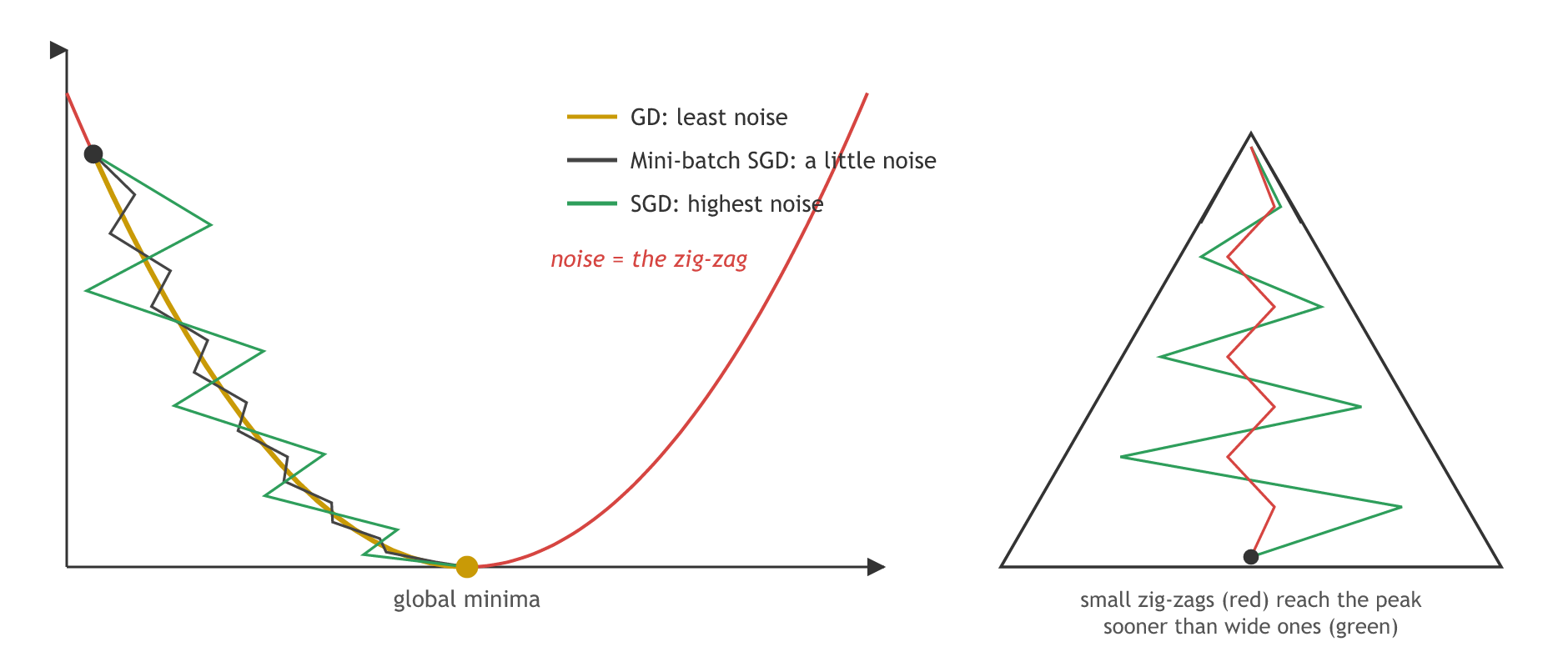
The board draws all three on one loss curve from the same starting point. Gradient descent (yellow) goes smoothly down to the global minima. SGD (green) jumps from side to side, because every update uses a single record. Mini-batch SGD (white on the board) zig-zags less. This zig-zag movement is called noise: SGD has the most, gradient descent the least, and mini-batch SGD a little, but it is still there.
The video's mountain analogy: you want to reach the peak. Walking straight there is fastest. Zig-zagging wide across the slope (the green person) takes a long time. Small zig-zags get there better than the green person. Training is the same climb, turned upside down, towards the global minima.
Training with three batch sizes
The same 1,000 records as in the gradient descent lesson, with batch sizes 1,000 (gradient descent), 50 (mini-batch SGD) and 1 (SGD).
import numpy as np

rng = np.random.default_rng(42)
n = 1000                                     # 1,000 records stand in for the board's 1,000,000
x = rng.uniform(0, 2, n)
y = 3 * x + 2 + rng.normal(0, 0.5, n) # the true line has w = 3 and b = 2def gradients(w, b, xb, yb):
error = w * xb + b - yb # ŷ − y for every record in the batch
return np.mean(error * xb), np.mean(error) # ∂C/∂w and ∂C/∂b
def cost(w, b):
return np.mean((w * x + b - y) ** 2) / 2 # C = 1/(2n) Σ (y − ŷ)²Splitting every epoch into batches
permutation shuffles the records at the start of each epoch, and the slice idx[start:start + batch_size] takes the next batch. Every batch is one iteration. The function returns every (w, b) the weights pass through.
def train(batch_size, updates, lr=0.1, seed=0):
    order = np.random.default_rng(seed)
    w, b, path, done = -1.0, -1.0, [(-1.0, -1.0)], 0
    while done < updates:
        idx = order.permutation(n)                   # shuffle the records every epoch
        for start in range(0, n, batch_size):
            batch = idx[start:start + batch_size]    # one batch = one iteration
            gw, gb = gradients(w, b, x[batch], y[batch])
            w, b = w - lr * gw, b - lr * gb
            path.append((w, b)); done += 1
            if done == updates:
                break
    return np.array(path)
Running 100 updates each
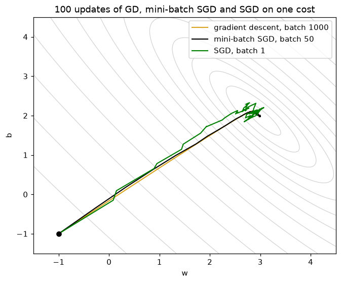
Each optimizer gets the same 100 weight updates, from w = −1, b = −1, with η = 0.1. The plot draws the three paths over the cost's contour lines.
import matplotlib.pyplot as plt

runs = [("gradient descent, batch 1000", 1000, "goldenrod"),
        ("mini-batch SGD, batch 50", 50, "black"), ("SGD, batch 1", 1, "green")]
fig, ax = plt.subplots(figsize=(7, 5.5))
W, B = np.meshgrid(np.linspace(-1.5, 4.5, 121), np.linspace(-1.5, 4.5, 121))
C = np.vectorize(cost)(W, B)
ax.contour(W, B, C, levels=np.geomspace(0.15, 20, 14), colors="lightgray", linewidths=0.8)
for name, batch_size, color in runs:
    path = train(batch_size, updates=100)
    steps = np.linalg.norm(np.diff(path, axis=0), axis=1).sum()   # total distance walked
    print(f"{name:29} records read {100 * batch_size:>7,}  w = {path[-1, 0]:.3f}  b = {path[-1, 1]:.3f}"
          f"  cost = {cost(*path[-1]):.4f}  path length = {steps:.2f}")
    ax.plot(path[:, 0], path[:, 1], color=color, lw=1.4, label=name)
ax.plot(-1, -1, "ko"); ax.set_xlabel("w"); ax.set_ylabel("b")
ax.set_title("100 updates of GD, mini-batch SGD and SGD on one cost")
ax.legend(); plt.show()gradient descent, batch 1000 records read 100,000 w = 2.997 b = 1.974 cost = 0.1286 path length = 5.16 mini-batch SGD, batch 50 records read 5,000 w = 3.000 b = 1.976 cost = 0.1286 path length = 5.69 SGD, batch 1 records read 100 w = 2.955 b = 2.076 cost = 0.1321 path length = 10.44
What the three paths show
- Gradient descent read 100,000 records for its 100 updates, mini-batch SGD 5,000 and SGD only 100. Per update, SGD is a thousand times cheaper than gradient descent here.
- Gradient descent and mini-batch SGD end at the same cost, 0.1286. A batch of 50 records already gives a good average of the gradient.
- SGD ends higher, and its path is about twice as long as the others: the extra distance is the zig-zag, the noise, spent walking sideways.
- The shapes match the board: smooth for gradient descent, a little wiggle for mini-batch SGD, wide zig-zags for SGD.
Setting the batch size in Keras
In Keras the batch size is an argument of fit, not of the optimizer, and the same optimizer object runs any of the three:
model.fit(X, y, epochs=100, batch_size=len(X))   # gradient descent: 1 iteration per epoch
model.fit(X, y, epochs=100, batch_size=1)        # SGD: one record per iteration
model.fit(X, y, epochs=100, batch_size=32)       # mini-batch SGD (32 if you leave batch_size out)
GD vs SGD vs mini-batch SGD
| Gradient descent | SGD | Mini-batch SGD | |
|---|---|---|---|
| Records per iteration | all (1,000,000) | 1 | batch size (1,000) |
| Iterations per epoch | 1 | 1,000,000 | 1,000 |
| Memory per update | huge RAM, often GPUs | very small | small |
| Noise in the path | least | highest | a little |
| Convergence | smooth, but each update is expensive | very slow, many noisy updates | better than SGD |
Where you use mini-batch SGD
- Almost every deep learning model: Keras trains in mini-batches by default, and batch sizes from about 32 to 256 are common (the materials' optimizer notebook gives 50 to 256).
- Data that does not fit in memory, such as millions of images, streamed one batch at a time from disk.
- Online learning, where SGD with a batch of 1 updates the model as each new record arrives.
permutation does this in the code above; Keras's fit shuffles by default.Related
- Previous: Gradient descent
- Next: SGD with momentum
- Add a fourth run with
batch_size=10: its path length lands between SGD and mini-batch SGD. - Give SGD 1,000 updates instead of 100, one full epoch, with
updates=1000 if batch_size == 1 else 100: its path length jumps to about 67 and its cost is still above 0.13, because SGD keeps bouncing around the minimum instead of settling. - Remove the shuffle by replacing
order.permutation(n)withnp.arange(n); the records are unsorted here, so little changes, but on sorted data this line matters.
Little by little, you're building something great.