Training and evaluating an ANN
Training and evaluating an ANN is the step that runs fit() over the training data epoch after epoch, stops when the validation loss stops improving, and then scores the trained network on the test set.
Last updated: 05 Oct, 2026 · TensorFlow 2 / Keras
Building an ANN in Keras compiled a network of 271 untrained parameters. Here the video trains it on the 8,000 churn customers, learns why a fixed number of epochs is a guess, and reads its predictions.
Fitting with validation_split and batch_size
fit() takes the training data and three settings. validation_split=0.33 holds part of X_train back to check the model on rows it does not train on. batch_size=10 updates the weights after every 10 rows, the mini-batch of SGD and mini-batch gradient descent. epochs=1000 runs a thousand passes over the data, which the video chooses to show why a better way to stop is needed.
model_history=classifier.fit(X_train,y_train,validation_split=0.33,batch_size=10,epochs=1000)Every epoch prints 536 steps and, as training goes on, the loss and validation loss fall while both accuracies rise: about 86% accuracy and 85% validation accuracy after a few minutes. The first epoch of the video's run shows a loss of 0.4260, an accuracy of 0.8112 and a validation loss of 0.3903. By epoch 31 to 44 the accuracy only moves around 86.4%, 86.3%, 86.1%, and the video stops the cell by hand.
The video calls the validation split cross validation and says it takes about 66% of the data per epoch. It is a single hold-out: Keras takes the last 33% of the rows of X_train, before any shuffling, as one fixed validation set and trains on the first 67% in every epoch. The code shows where the 536 comes from.
import math

n_train = 8000                         # rows of X_train
split_at = int(math.floor(n_train * (1.0 - 0.33)))   # how Keras splits: the first 67% train
print("training rows: 0 to", split_at - 1, "->", split_at, "rows")
print("validation rows:", split_at, "to", n_train - 1, "->", n_train - split_at, "rows")
print("steps per epoch, batch_size=10:", math.ceil(split_at / 10))
print("steps per epoch, batch_size=32:", math.ceil(split_at / 32))
print("2024 run, all 8000 rows, batch 32:", math.ceil(n_train / 32))training rows: 0 to 5358 -> 5359 rows validation rows: 5359 to 7999 -> 2641 rows steps per epoch, batch_size=10: 536 steps per epoch, batch_size=32: 168 2024 run, all 8000 rows, batch 32: 250
- 5,359 rows train and 2,641 validate: 8000 × 0.67 is 5,360, but in floating point 1 − 0.33 is a hair below 0.67, and Keras rounds the product down.
- 536 steps per epoch is 5,359 rows in batches of 10, the last batch holding 9 rows. With Keras's default batch_size of 32 it would be 168.
- The 2024 run's 250 steps are its 8,000 rows in batches of 32: it passes the test set as
validation_datainstead of splitting X_train.
Stopping early on the validation loss
Early stopping answers the question of how many epochs to train: it watches a metric after every epoch and stops training when that metric stops improving. The video copies the EarlyStopping signature from the Keras documentation and sets its values.
## Early Stopping
import tensorflow as tf
early_stopping=tf.keras.callbacks.EarlyStopping(
    monitor="val_loss",
    min_delta=0.0001,
    patience=20,
    verbose=1,
    mode="auto",
    baseline=None,
    restore_best_weights=False,
)- monitor="val_loss": watch the validation loss.
- min_delta=0.0001: a fall smaller than this does not count as an improvement.
- patience=20: stop after 20 epochs in a row without an improvement.
- verbose=1: print a line when it stops.
- restore_best_weights=False: keep the weights of the last epoch, not of the best one.
The callback goes into fit() through callbacks. The video passes the object itself; Keras also accepts a list, callbacks=[early_stopping], which is the usual form and lets you add more callbacks.
Reading the early-stopping run
After a kernel restart, the video re-runs the cells in order (layers, opt, compile with optimizer=opt, the callback) and trains again.
model_history=classifier.fit(X_train,y_train,validation_split=0.33,batch_size=10,epochs=1000,callbacks=early_stopping)... Epoch 29/1000 536/536 [==============================] - 3s 5ms/step - loss: 0.3308 - accuracy: 0.8666 - val_loss: 0.3891 - val_accuracy: 0.8512 Epoch 30/1000 536/536 [==============================] - 3s 5ms/step - loss: 0.3296 - accuracy: 0.8662 - val_loss: 0.3681 - val_accuracy: 0.8527 Epoch 30: early stopping
Training ends by itself at epoch 30 with about 85% validation accuracy. model_history.history keeps one list per metric, one value per epoch:
model_history.history.keys()dict_keys(['loss', 'accuracy', 'val_loss', 'val_accuracy'])
The video plots the accuracy and the loss of the two splits. Its plot code labels the second line 'test', but that line is the validation split; the test set is used only for the predictions below.
# summarize history for loss
plt.plot(model_history.history['loss'])
plt.plot(model_history.history['val_loss'])
plt.title('model loss')
plt.ylabel('loss')
plt.xlabel('epoch')
plt.legend(['train', 'test'], loc='upper left')
plt.show()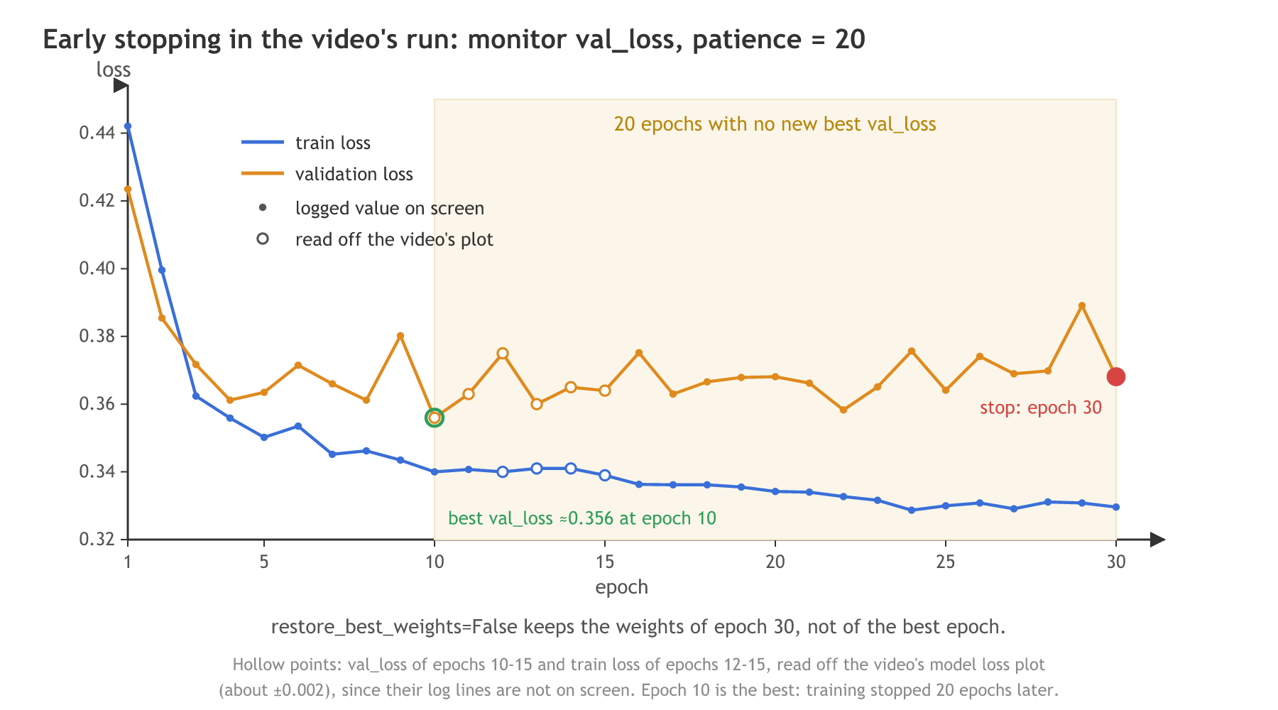
- The training loss keeps falling, from 0.4421 in epoch 1 to 0.3296 in epoch 30.
- The validation loss is lowest at epoch 10, about 0.356 on the plot (that log line is hidden on screen), and then moves between 0.358 and 0.389. The widening gap between the two curves is the start of overfitting.
- Epoch 30 = the best epoch + 20: with patience=20, the 20 epochs after the best one without a new best end the run.
- The model evaluated next is the epoch-30 model, since restore_best_weights=False. With True, Keras would go back to the weights of the best epoch.
Replaying early stopping on the 2024 run
The 2024 version uses patience=10 and restore_best_weights=True, with the test set as validation data:
## Set up Early Stopping
early_stopping_callback=EarlyStopping(monitor='val_loss',patience=10,restore_best_weights=True)### Train the model
history=model.fit(
X_train,y_train,validation_data=(X_test,y_test),epochs=100,
callbacks=[tensorflow_callback,early_stopping_callback]
)Epoch 1/100 250/250 [==============================] - 1s 3ms/step - loss: 0.3496 - accuracy: 0.8591 - val_loss: 0.3424 - val_accuracy: 0.8595 Epoch 2/100 250/250 [==============================] - 1s 3ms/step - loss: 0.3426 - accuracy: 0.8622 - val_loss: 0.3427 - val_accuracy: 0.8580 Epoch 3/100 250/250 [==============================] - 1s 2ms/step - loss: 0.3397 - accuracy: 0.8630 - val_loss: 0.3508 - val_accuracy: 0.8605 Epoch 4/100 250/250 [==============================] - 1s 2ms/step - loss: 0.3406 - accuracy: 0.8622 - val_loss: 0.3583 - val_accuracy: 0.8590 Epoch 5/100 250/250 [==============================] - 1s 2ms/step - loss: 0.3378 - accuracy: 0.8626 - val_loss: 0.3424 - val_accuracy: 0.8555 Epoch 6/100 250/250 [==============================] - 1s 3ms/step - loss: 0.3322 - accuracy: 0.8654 - val_loss: 0.3423 - val_accuracy: 0.8600 Epoch 7/100 250/250 [==============================] - 1s 2ms/step - loss: 0.3311 - accuracy: 0.8661 - val_loss: 0.3412 - val_accuracy: 0.8605 Epoch 8/100 250/250 [==============================] - 1s 2ms/step - loss: 0.3256 - accuracy: 0.8665 - val_loss: 0.3515 - val_accuracy: 0.8540 Epoch 9/100 250/250 [==============================] - 1s 2ms/step - loss: 0.3280 - accuracy: 0.8665 - val_loss: 0.3623 - val_accuracy: 0.8540 Epoch 10/100 250/250 [==============================] - 1s 2ms/step - loss: 0.3251 - accuracy: 0.8677 - val_loss: 0.3474 - val_accuracy: 0.8540 Epoch 11/100 250/250 [==============================] - 1s 2ms/step - loss: 0.3227 - accuracy: 0.8690 - val_loss: 0.3571 - val_accuracy: 0.8565 Epoch 12/100 250/250 [==============================] - 1s 2ms/step - loss: 0.3216 - accuracy: 0.8664 - val_loss: 0.3565 - val_accuracy: 0.8550 Epoch 13/100 250/250 [==============================] - 1s 3ms/step - loss: 0.3171 - accuracy: 0.8699 - val_loss: 0.3569 - val_accuracy: 0.8570 Epoch 14/100 250/250 [==============================] - 1s 3ms/step - loss: 0.3141 - accuracy: 0.8689 - val_loss: 0.3562 - val_accuracy: 0.8605 Epoch 15/100 250/250 [==============================] - 1s 3ms/step - loss: 0.3141 - accuracy: 0.8704 - val_loss: 0.3554 - val_accuracy: 0.8600 Epoch 16/100 250/250 [==============================] - 1s 2ms/step - loss: 0.3115 - accuracy: 0.8733 - val_loss: 0.3585 - val_accuracy: 0.8555 Epoch 17/100 250/250 [==============================] - 1s 2ms/step - loss: 0.3081 - accuracy: 0.8725 - val_loss: 0.3636 - val_accuracy: 0.8535
Its first epoch already shows 86% accuracy, which a fresh network does not reach; the cell was most likely run on a model that had been trained before. Using the test set for early stopping also lets the test data steer training a little; a separate validation set avoids that. The rule itself is easy to replay on its 17 saved validation losses:
val_loss = [0.3424, 0.3427, 0.3508, 0.3583, 0.3424, 0.3423, 0.3412, 0.3515, 0.3623,
            0.3474, 0.3571, 0.3565, 0.3569, 0.3562, 0.3554, 0.3585, 0.3636]   # the 2024 run
patience, min_delta = 10, 0.0

best, best_epoch, wait = float("inf"), 0, 0
for epoch, v in enumerate(val_loss, start=1):
    wait += 1
    if v < best - min_delta:           # an improvement resets the count
        best, best_epoch, wait = v, epoch, 0
    if wait >= patience:
        print(f"stop after epoch {epoch}: {wait} epochs since the best")
        break
print(f"best val_loss {best} at epoch {best_epoch}")
print("restore_best_weights=True keeps epoch", best_epoch, "; False keeps epoch", epoch)stop after epoch 17: 10 epochs since the best best val_loss 0.3412 at epoch 7 restore_best_weights=True keeps epoch 7 ; False keeps epoch 17
- The best val_loss is 0.3412 at epoch 7; epochs 8 to 17 bring no lower value.
- Training stops after epoch 17, the 10th epoch without an improvement: the same epoch at which the 2024 run stopped.
- restore_best_weights=True hands back the epoch-7 weights instead of the epoch-17 ones.
Predicting and scoring the test set
classifier.predict(X_test) returns one probability per test customer. A probability of 0.5 or more becomes True (leaves) and anything below becomes False (stays). The Confusion matrix counts the four combinations of true and predicted class.
# Part 3 - Making the predictions and evaluating the model

# Predicting the Test set results
y_pred = classifier.predict(X_test)
y_pred = (y_pred >= 0.5)## make the confusion matrix
from sklearn.metrics import confusion_matrix
cm=confusion_matrix(y_test,y_pred)
cmarray([[1527, 68],
[ 215, 190]])## Calculate the accuracy
from sklearn.metrics import accuracy_score
score=accuracy_score(y_pred,y_test)score0.8585
accuracy_score expects the true labels first, accuracy_score(y_test, y_pred); accuracy gives the same number either way round, but precision and recall would not. The video's 0.8585 is (1527 + 190) / 2000, and it notes that a run may give 86% or 87%: the starting weights are random, so every run differs slightly.
import numpy as np

cm = np.array([[1527, 68],
               [215, 190]])            # the video's confusion matrix
tn, fp, fn, tp = cm.ravel()
total = cm.sum()
print("test customers:", total, "| stayed:", tn + fp, "| left:", fn + tp)
print("accuracy:", (tn + tp) / total)
print("always predicting 'stays':", (tn + fp) / total)
print("precision for 'leaves':", round(tp / (tp + fp), 4))
print("recall for 'leaves':", round(tp / (tp + fn), 4))test customers: 2000 | stayed: 1595 | left: 405 accuracy: 0.8585 always predicting 'stays': 0.7975 precision for 'leaves': 0.7364 recall for 'leaves': 0.4691
- Accuracy 0.8585 on 2,000 test customers, 1,595 of whom stayed and 405 left.
- Always predicting "stays" scores 0.7975, so the network adds about 6 points over doing nothing.
- Precision 0.7364: when the network says a customer will leave, it is right about three times in four.
- Recall 0.4691: it finds fewer than half of the customers who leave. With 20% churners, a threshold below 0.5 or class weights would trade some precision for recall; Precision, recall and F-beta covers the trade.
classifier.get_weights() returns the trained arrays in order: kernel (11, 11) and bias (11,), kernel (11, 7) and bias (7,), kernel (7, 6) and bias (6,), kernel (6, 1) and bias (1,), the 271 parameters counted before. The values differ on every run.
Adding dropout layers to the network
The video then adds the regularization of Dropout. It first tries Dense(units=7, activation='relu', dropout=0.3), which fails because Dense has no dropout argument (Keras 3 says "Unrecognized keyword arguments passed to Dense"), then classifier.add(Dropout=0.3), which fails because add() takes a layer. Dropout(0.2) is a layer of its own, added after the layer whose outputs it drops. The clean version, rebuilt from Sequential():
classifier=Sequential()
classifier.add(Dense(units=11,activation='relu'))
classifier.add(Dense(units=7,activation='relu'))
classifier.add(Dropout(0.2))
classifier.add(Dense(units=6,activation='relu'))
classifier.add(Dropout(0.3))
classifier.add(Dense(1,activation='sigmoid'))
classifier.compile(optimizer=opt,loss='binary_crossentropy',metrics=['accuracy'])
model_history=classifier.fit(X_train,y_train,validation_split=0.33,batch_size=10,epochs=1000,callbacks=[early_stopping])
With dropout the first epoch starts lower, loss 0.4809, accuracy 0.7994 and validation loss 0.4466 in the video's run, because a fifth to a third of the hidden outputs are switched off on every step. In the video, one of the failed cells had already added a Dense(units=7) before raising its error, so its dropout model had two layers of 7. Starting again from Sequential(), as above, avoids that.
The video ends by saying the trained model can be saved with pickle or in the h5 format. On current Keras, classifier.save('churn_model.keras') writes the native format and tf.keras.models.load_model('churn_model.keras') reads it back; .h5 still works but is marked legacy.
validation_split vs validation_data
| validation_split=0.33 | validation_data=(X_val, y_val) | |
|---|---|---|
| Where the rows come from | the last 33% of X_train, before shuffling | a set you pass in |
| Rows left for training | 67% of X_train | all of X_train |
| Used in | the video's run (536 steps of 10) | the 2024 run (250 steps of 32) |
| Risk | the last rows may not be a random sample if the data is sorted | passing the test set makes it a validation set |
Where you use early stopping
- Any training run where the right number of epochs is unknown: set a large
epochsand let the validation loss decide. - Comparing models fairly, each stopped at its own best point with
restore_best_weights=True. - Saving compute on long runs, together with a ModelCheckpoint callback that writes the best model to disk.
restore_best_weights=False, the default, the model you get back is the one from the epoch training stopped, which is patience epochs past the best one and often worse. In the video's run that is epoch 30 instead of epoch 10. Set it to True unless you want the last weights.Related
- Previous: Building an ANN in Keras
- Next: Hidden layers and neurons with Keras Tuner
- See also: Confusion matrix, Dropout
- Reference: EarlyStopping in the Keras API
- In the replay, set
patience = 5and find the epoch at which training would stop. - Set
min_delta = 0.001in the replay and check whether epoch 7's 0.3412 still counts as an improvement over 0.3424. - In the confusion-matrix run, move 50 customers from the false-negative cell to the true-positive cell and see how recall and accuracy change.
Every expert started right here.