Convolution and filters
Convolution is an operation that slides a small grid of weights, the filter or kernel, over an image and writes the sum of the cell-by-cell products at each position into a new grid called a feature map.
Last updated: 05 Oct, 2026 · NumPy
It is the first step of every CNN in Convolutional neural networks (CNN). A filter that matches a pattern, such as a vertical edge, gives large values where the pattern is and zeros where it is not.
Sliding a 3×3 filter over a 6×6 image
The board's image is 6×6: three columns of 0 (black) and three of 255 (white). The first step divides every pixel by 255, which turns the image into three columns of 0 and three of 1. The video calls this min max scaling; dividing by 255 equals min-max scaling only when the darkest pixel is 0 and the brightest 255, so it is usually called normalising or rescaling.
A 3×3 filter is placed on the top-left corner. Each filter value is multiplied by the pixel under it, the nine products are added, and the sum goes into the first cell of the output. The filter then moves one cell to the right, which is a stride of 1, and repeats; at the end of a row it moves one cell down. A 3×3 filter fits in 4 positions across a 6-pixel row, so the output is 4×4.
The first filter on the board is 1 2 1 / 0 0 0 / −1 −2 −1, the horizontal edge filter. The board writes rows of −4 for it; on this image every window sums to 0, because all rows of the image are the same and the +1 +2 +1 row cancels the −1 −2 −1 row. A 4×4 of zeros is the right answer: the image has no horizontal edge.
Finding the vertical edge
The new filter is 1 0 −1 / 2 0 −2 / 1 0 −1, the vertical edge filter. In the first position every pixel under it is 0, so the sum is 0. One step to the right, the right column of the filter (−1, −2, −1) sits on 1s and the rest on 0s, so the sum is −4. The third position also gives −4, and the fourth is 0 again. Every row of the image is the same, so every row of the output is 0 −4 −4 0.
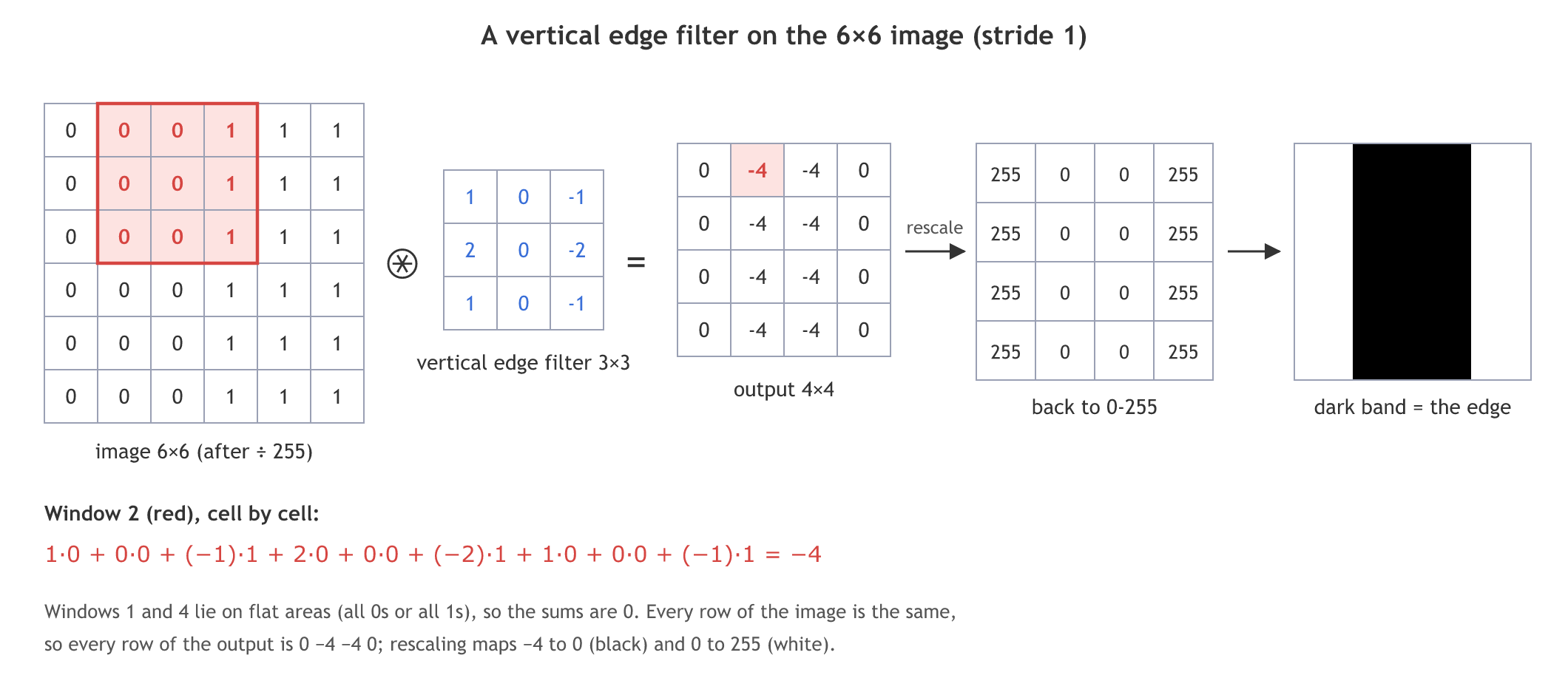
To see the result as an image, the output goes back to the 0-255 range: the lowest value (−4) becomes 0 and the highest (0) becomes 255, so each row reads 255 0 0 255. 255 is white and 0 is black, so the picture is white on both sides with a black band in the middle: the vertical edge, where the image changes from 0 to 1.
The clip ends by comparing the filter with the V1 to V7 layers, each extracting one kind of information, and by calling this a correlation operation. That is the precise name: the sum above, with the filter not flipped, is cross-correlation, and it is what Keras Conv2D computes. Convolution in mathematics flips the filter first; for filters that are learned the difference does not matter.
The edge comes out dark because the image goes from dark (0) on the left to light (1) on the right, which makes the sums negative there. On an image that goes from light to dark, the same filter gives +4 and the edge shows white.
Learning the filter values with backpropagation
A real CNN does not hard-code filters. As with the weights of an ANN, the filter values start random and are updated by backpropagation (Backpropagation and weight update), so the network finds the filters that suit its images. A layer holds many filters, for horizontal edges, vertical edges, round shapes and more, and each filter gives its own output.
After the convolution, a ReLU activation, max(0, x), is applied to every value of the output. Its derivative is easy to find, which backpropagation needs to update the filters; other activations such as PReLU also work (ReLU and its variants).
The clip also changes the stride to 2 and writes the output size as (n + 2p − f + 1) / s; the correct formula is ⌊(n + 2p − f) / s⌋ + 1, worked through in Padding and stride.
In a real layer ReLU acts on the raw output 0 −4 −4 0, which gives all zeros: this filter's edge would vanish. A learned filter can take the opposite sign, −1 0 1 / −2 0 2 / −1 0 1, and give +4, which ReLU keeps. Training settles on whichever sign is useful.
Convolving an RGB image
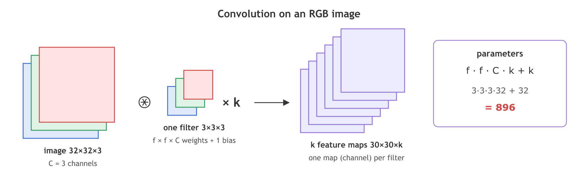
The video shows RGB images but convolves only the grayscale one. For an image with C channels, each filter is f×f×C: one f×f slice per channel. At each position all f·f·C products are added, plus one bias, giving a single number, so one filter always gives one 2-D feature map. A layer of k filters gives k feature maps, stacked as the k channels of the output.
The CIFAR-10 model in CNN in Keras starts with 32 filters of 3×3 on 3 channels: 3·3·3·32 + 32 = 896 parameters. VGG16's first layer has 64 filters: 3·3·3·64 + 64 = 1,792, and its second layer, on 64 channels, 3·3·64·64 + 64 = 36,928.
Running the 6×6 example in NumPy
The convolution function
Two loops place the filter at every position; at each one the window is multiplied cell by cell with the filter and summed.
def conv2d(img, k):
    f = k.shape[0]
    n = img.shape[0] - f + 1                       # n - f + 1
    out = np.zeros((n, n))
    for i in range(n):
        for j in range(n):
            out[i, j] = (img[i:i + f, j:j + f] * k).sum()   # multiply cell by cell, add
    return out
The two filters and the rescaling
vertical = np.array([[1, 0, -1], [2, 0, -2], [1, 0, -1]])
horizontal = np.array([[1, 2, 1], [0, 0, 0], [-1, -2, -1]])
v = conv2d(img, vertical)
rescaled = (v - v.min()) / (v.max() - v.min()) * 255   # -4 -> 0, 0 -> 255
Filters over three channels
For RGB, each filter's three slices are applied to the three channels and the results added, which gives one map per filter.
maps = np.stack([sum(conv2d(rgb[:, :, c], w[:, :, c]) for c in range(3))
                 for w in filters], axis=-1)        # one map per filter, stacked
The vertical and horizontal filters on the board's image
import numpy as np
from scipy.signal import correlate2d

def conv2d(img, k):
    f = k.shape[0]
    n = img.shape[0] - f + 1                       # n - f + 1
    out = np.zeros((n, n))
    for i in range(n):
        for j in range(n):
            out[i, j] = (img[i:i + f, j:j + f] * k).sum()   # multiply cell by cell, add
    return out

img = np.array([[0, 0, 0, 255, 255, 255]] * 6) / 255     # the 6x6 image, scaled to 0-1
vertical = np.array([[1, 0, -1], [2, 0, -2], [1, 0, -1]])
horizontal = np.array([[1, 2, 1], [0, 0, 0], [-1, -2, -1]])

v = conv2d(img, vertical)
print("vertical filter:")
print(v.astype(int))
print("rescaled to 0-255:")
print(((v - v.min()) / (v.max() - v.min()) * 255).astype(int))
print("horizontal filter:")
print(conv2d(img, horizontal).astype(int))
print("ReLU of the vertical map, row 1:", np.maximum(0, v)[0])
print("ReLU with the filter's sign flipped:", np.maximum(0, conv2d(img, -vertical))[0])
print("same as scipy correlate2d:", np.allclose(v, correlate2d(img, vertical, mode="valid")))

rgb = np.random.default_rng(0).random((32, 32, 3))                 # a random 32x32 RGB image
filters = np.random.default_rng(1).standard_normal((32, 3, 3, 3))  # k = 32 filters, each 3x3x3
maps = np.stack([sum(conv2d(rgb[:, :, c], w[:, :, c]) for c in range(3)) for w in filters], axis=-1)
print("RGB output shape:", maps.shape, " parameters:", filters.size + len(filters))vertical filter: [[ 0 -4 -4 0] [ 0 -4 -4 0] [ 0 -4 -4 0] [ 0 -4 -4 0]] rescaled to 0-255: [[255 0 0 255] [255 0 0 255] [255 0 0 255] [255 0 0 255]] horizontal filter: [[0 0 0 0] [0 0 0 0] [0 0 0 0] [0 0 0 0]] ReLU of the vertical map, row 1: [0. 0. 0. 0.] ReLU with the filter's sign flipped: [0. 4. 4. 0.] same as scipy correlate2d: True RGB output shape: (30, 30, 32) parameters: 896
What the feature maps show
- The vertical filter gives 0 −4 −4 0 in every row, the board's values, and rescaling turns them into 255 0 0 255.
- The horizontal filter gives a 4×4 of zeros: the image has no horizontal edge, so the board's rows of −4 do not appear.
- ReLU on the raw map leaves only zeros, while the filter with its sign flipped gives 0 4 4 0, which ReLU keeps.
- scipy's correlate2d agrees with the two loops, which confirms that a CNN's convolution is cross-correlation.
- 32 filters on a 32×32×3 image give an output of shape (30, 30, 32) and 896 parameters, the numbers of the first layer in the CIFAR-10 model.
Vertical vs horizontal edge filter
| Vertical edge filter | Horizontal edge filter | |
|---|---|---|
| Values | 1 0 −1 / 2 0 −2 / 1 0 −1 | 1 2 1 / 0 0 0 / −1 −2 −1 |
| Responds to | a change from left to right | a change from top to bottom |
| On the 6×6 image | 0 −4 −4 0 in each row | all zeros |
| After rescaling | 255 0 0 255: a dark vertical band | no edge to show |
| Classic name | Sobel x filter | Sobel y filter |
Where you use convolution
- The first layers of every CNN, where learned filters play the role of these hand-made edge filters.
- Classic image processing: the two filters here are the Sobel filters, used for edge detection in tools such as OpenCV.
- Blurring and sharpening: a 3×3 filter of equal weights 1/9 blurs an image, and a filter with a large centre value sharpens it.
Related
- Previous: Convolutional neural networks (CNN)
- Next: Padding and stride
- See also: Backpropagation and weight update
- See also: ReLU and its variants
- Use the image
[[255, 255, 255, 0, 0, 0]] * 6(light to dark) and check that the vertical filter now gives 0 4 4 0. - Transpose the image with
img.Tand run the horizontal filter on it: the edge is now horizontal, so the zeros turn into −4s. - Change the number of filters from 32 to 64 and check that the parameter count becomes 1,792 as in VGG16's first layer.
This is what real progress feels like.