Weight initialization
Weight initialization is the step that sets every weight of a neural network to a starting value before training, chosen small, different from neuron to neuron and with a spread that suits the layer's size.
Last updated: 05 Oct, 2026 · NumPy
The Adam optimizer decides how the weights move during training. Where they start decides whether training gets going at all: weights that start too large make the gradients explode, weights that start identical make every neuron learn the same thing. The notes in the video's materials repo cover it in three pages: the problem large weights cause, three key points for good starting weights and three families of techniques.
Starting all the weights at zero
The Weights and bias lesson asks what happens if every weight starts at 0: x1 × 0, x2 × 0 and x3 × 0 are all 0, so the neuron passes on nothing. The video adds a bias to get round that. A bias does not fix the deeper problem, though. If all the weights into a layer are equal, zero or not, every neuron in the layer computes the same output, gets the same gradient and receives the same update. They stay copies of each other for the whole of training, so a layer of 100 neurons learns no more than one neuron. This is the symmetry problem, and random starting weights are what break it.
Backpropagating once from equal weights
The code runs one record with three inputs through a 3-3-1 network of sigmoid neurons and computes the gradient of every first-layer weight, once with all weights at 0 and once with all at 0.5.
h = 1 / (1 + np.exp(-(x @ W1)))         # hidden layer of 3 sigmoid neurons
d_h = (W2[:, 0] * d_out) * h * (1 - h)  # error reaching each hidden neuron
gW1 = np.outer(x, d_h) # one gradient per weight, column = neuronimport numpy as np
x = np.array([1.0, 2.0, 3.0]) # one record with 3 inputs
y = 1.0 # its label
for name, W1, W2 in [("all zeros", np.zeros((3, 3)), np.zeros((3, 1))),
("all 0.5", np.full((3, 3), 0.5), np.full((3, 1), 0.5))]:
h = 1 / (1 + np.exp(-(x @ W1))) # hidden layer of 3 sigmoid neurons
yhat = 1 / (1 + np.exp(-(h @ W2))) # output neuron
d_out = yhat - y # dL/dz at the output (log loss + sigmoid)
d_h = (W2[:, 0] * d_out) * h * (1 - h)
gW1 = np.outer(x, d_h) # gradient for every weight into the hidden layer
print(name, "| hidden outputs:", np.round(h, 4))
print("gradient of W1, one column per hidden neuron:")
print(np.round(gW1, 4))all zeros | hidden outputs: [0.5 0.5 0.5] gradient of W1, one column per hidden neuron: [[-0. -0. -0.] [-0. -0. -0.] [-0. -0. -0.]] all 0.5 | hidden outputs: [0.9526 0.9526 0.9526] gradient of W1, one column per hidden neuron: [[-0.0044 -0.0044 -0.0044] [-0.0087 -0.0087 -0.0087] [-0.0131 -0.0131 -0.0131]]
- All zeros: the three hidden neurons all output 0.5 (the sigmoid of 0) and every first-layer gradient is 0, because the zero weights into the output send no error back. The output weights do get a gradient, the same −0.25 for each, so from the next step the first-layer weights start to move, but in lockstep, like the 0.5 case below.
- All 0.5: the gradients are not zero, but the three columns are identical (−0.0044, −0.0087, −0.0131). Every hidden neuron gets the same update and stays a copy of the others.
Exploding gradients from large weights
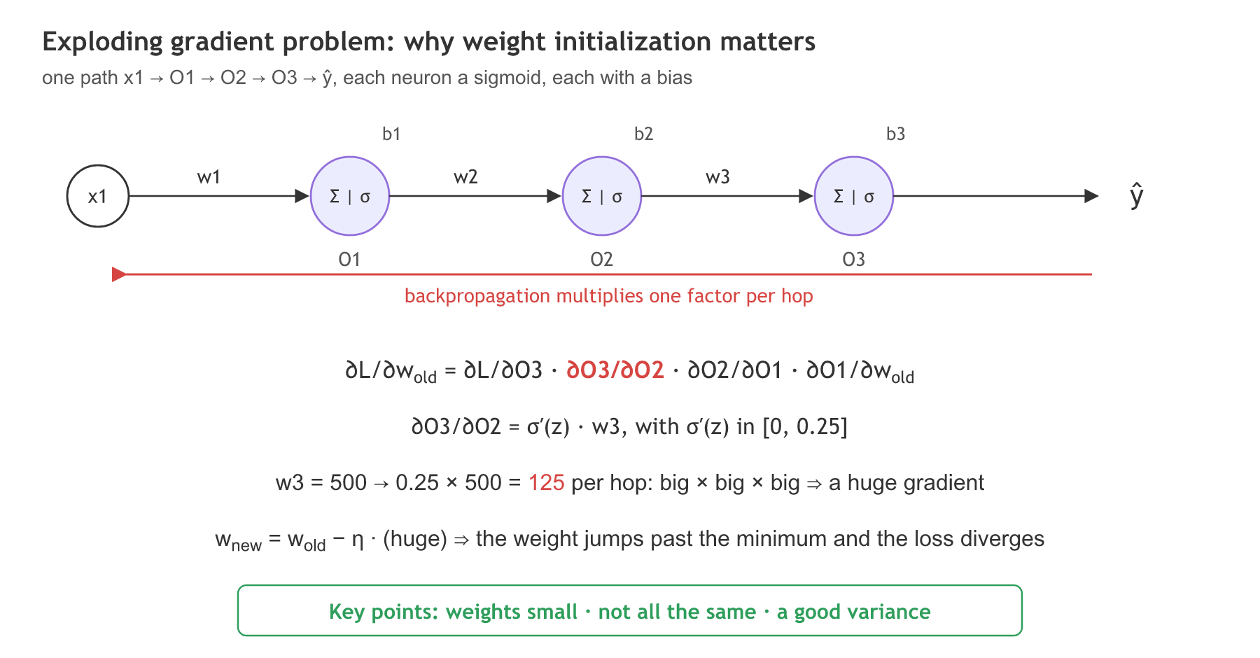
The notes open with the opposite problem. Take one path x1 → O1 → O2 → O3 → ŷ, each neuron a sigmoid with its own bias. Backpropagation updates a weight with wnew = wold − η · ∂L/∂wold, and the Chain rule of derivatives writes that slope as one factor per hop:
Each middle factor is the sigmoid's derivative times the next weight. With z = O2·w3 + b3:
In the Vanishing gradient problem lesson the weights were small, the factors were below 0.25 and the product shrank towards 0. Here the notes start w3 at 500 to 1000. Then one factor is up to 0.25 × 500 = 125, and big × big × big gives a huge slope. The update wnew = wold − η · (huge) jumps far past the minimum, the next slope is bigger still, and the loss zig-zags upward instead of settling. This is the exploding gradient problem, and its cause is weights that start with a very high value.
Following the three key points
The notes sum up both problems in three rules for the starting weights:
- Weights should be small, so the chain-rule factors do not blow up.
- Weights should not be the same, so neurons in a layer can learn different things.
- Weights should have a good variance: not so tiny that signals fade, not so wide that they explode. The right spread depends on how many inputs a neuron has.
Every technique below draws random weights (rule 2) centred on 0 (rule 1) with a spread computed from the layer's size (rule 3). Two numbers describe the size: input (fan-in), the number of neurons feeding the layer, and output (fan-out), the number of neurons it feeds. The notes draw two cases: a 1 → 3 → 1 network has input = 1 and output = 1 for its hidden layer, and a 3-3-3 network has input = 3 and output = 3.
Drawing weights from a uniform distribution
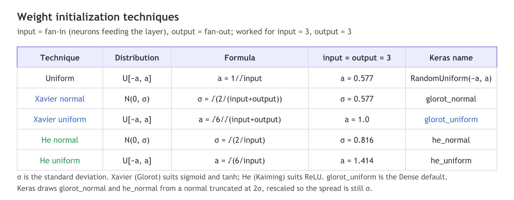
The simplest rule draws every weight Wij from a uniform distribution whose limit shrinks with the number of inputs. For three inputs that is the range [−1/√3, 1/√3], about ±0.577.
Using Xavier (Glorot) initialization
Xavier Glorot, the researcher the method is named after, worked out a spread that keeps the variance of the signal about the same going forward and the gradient going backward, which needs both the input and the output size. It comes in a normal and a uniform version. In N(0, σ) the σ is the standard deviation, not the variance.
Using He (Kaiming) initialization
Kaiming He's version is built for ReLU. ReLU sets about half of its inputs to 0, which halves the variance at every layer, so He doubles the variance to make up for it and uses only the input size.
Computing the limits for three inputs
The five formulas in NumPy
fan_in, fan_out = 3, 3
xavier_sigma = np.sqrt(2 / (fan_in + fan_out))        # normal: standard deviation
xavier_limit = np.sqrt(6) / np.sqrt(fan_in + fan_out)  # uniform: range [-a, a]
he_sigma, he_limit = np.sqrt(2 / fan_in), np.sqrt(6 / fan_in)
Checking the spread of uniform draws
rng.uniform(-a, a, size=...) draws weights from U[−a, a]. A uniform range has a standard deviation of a/√3, which the run compares with the draws.
import numpy as np

fan_in, fan_out = 3, 3                   # the 3-3-3 network of the notes
limits = {
    "uniform        a": 1 / np.sqrt(fan_in),
    "xavier normal  σ": np.sqrt(2 / (fan_in + fan_out)),
    "xavier uniform a": np.sqrt(6) / np.sqrt(fan_in + fan_out),
    "he normal      σ": np.sqrt(2 / fan_in),
    "he uniform     a": np.sqrt(6 / fan_in),
}
for name, v in limits.items():
    print(f"{name} = {v:.3f}")

rng = np.random.default_rng(0)
a = np.sqrt(6) / np.sqrt(fan_in + fan_out)
w = rng.uniform(-a, a, size=100_000)     # many Xavier-uniform draws
print("xavier uniform draws: min", w.min().round(3), "max", w.max().round(3), "std", w.std().round(3))
print("a / sqrt(3) =", round(a / np.sqrt(3), 3))uniform a = 0.577 xavier normal σ = 0.577 xavier uniform a = 1.000 he normal σ = 0.816 he uniform a = 1.414 xavier uniform draws: min -1.0 max 1.0 std 0.577 a / sqrt(3) = 0.577
- Uniform a = 0.577 is 1/√3, the notes' [−1/√3, 1/√3].
- Xavier normal σ = 0.577 and Xavier uniform a = 1.000: for input = output = 3, √(2/6) and √6/√6.
- He normal σ = 0.816 and He uniform a = 1.414 are √(2/3) and √2, larger than Xavier because He divides by the input size only.
- The uniform draws have a standard deviation of 0.577, the same as a/√3 and the same as the Xavier normal σ. The √6 in the uniform formula is there to make the two versions spread equally; the same holds for He (1.414/√3 = 0.816).
Measuring activations through ten layers
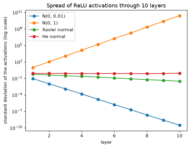
The point of a good variance shows up in a deep network. The code pushes 1000 random records through ten Dense layers of 256 ReLU neurons, starting the weights four ways, and prints the standard deviation of the activations after layers 1, 5 and 10.
a = x
for layer in range(10):
    a = np.maximum(0, a @ init(256, 256))   # one Dense layer + ReLU
stds.append(a.std()) # how spread out the signal isimport numpy as np
import matplotlib.pyplot as plt
rng = np.random.default_rng(0)
x = rng.standard_normal((1000, 256)) # 1000 records, 256 features
inits = {
"N(0, 0.01)": lambda fi, fo: rng.normal(0, 0.01, (fi, fo)),
"N(0, 1)": lambda fi, fo: rng.normal(0, 1.0, (fi, fo)),
"Xavier normal": lambda fi, fo: rng.normal(0, np.sqrt(2 / (fi + fo)), (fi, fo)),
"He normal": lambda fi, fo: rng.normal(0, np.sqrt(2 / fi), (fi, fo)),
}
for name, init in inits.items():
a, stds = x, []
for layer in range(10): # ten Dense layers of 256 ReLU neurons
a = np.maximum(0, a @ init(256, 256))
stds.append(a.std())
print(f"{name:14s} layer 1: {stds[0]:.3g} layer 5: {stds[4]:.3g} layer 10: {stds[9]:.3g}")
plt.semilogy(range(1, 11), stds, marker="o", label=name)
plt.title("Spread of ReLU activations through 10 layers")
plt.xlabel("layer")
plt.ylabel("standard deviation of the activations (log scale)")
plt.legend()
plt.show()N(0, 0.01) layer 1: 0.094 layer 5: 1.59e-05 layer 10: 3.04e-10 N(0, 1) layer 1: 9.39 layer 5: 1.54e+05 layer 10: 2.65e+10 Xavier normal layer 1: 0.584 layer 5: 0.175 layer 10: 0.0308 He normal layer 1: 0.826 layer 5: 0.771 layer 10: 0.865
What the ten layers show
- N(0, 0.01), small weights chosen without regard to the layer's size, shrinks the signal about 9 times per layer, to 3.04e-10 by layer 10. The later layers receive almost nothing, and the gradients flowing back shrink the same way.
- N(0, 1) grows it about 11 times per layer, to 2.65e+10: the exploding case from the notes, with weights that are too large for 256 inputs.
- Xavier normal keeps the first layer healthy (0.584) but loses about 30% of the spread at each ReLU layer, 0.175 by layer 5 and 0.0308 by layer 10. Xavier was designed for tanh and sigmoid, which do not zero half their inputs.
- He normal holds the spread near 0.8 at every depth (0.826, 0.771, 0.865). Doubling the variance makes up for the half that ReLU switches off.
Setting the initializer in Keras
In Keras each layer takes a kernel_initializer for its weights and a bias_initializer for its biases. The Dense page that the video opens in the ANN practical shows the defaults: kernel_initializer="glorot_uniform" and bias_initializer="zeros". Biases can start at 0 because the random weights already break the symmetry. The normal versions in Keras, glorot_normal and he_normal, draw from a truncated normal: values more than two standard deviations from 0 are drawn again, and the σ is scaled up so the spread still matches the formula.
from tensorflow.keras.layers import Dense

Dense(64, activation="relu", kernel_initializer="he_normal")      # ReLU layer: He
Dense(64, activation="tanh", kernel_initializer="glorot_normal")  # tanh layer: Xavier
Dense(1, activation="sigmoid")                 # default glorot_uniform, zero bias
Xavier vs He initialization
| Xavier (Glorot) | He (Kaiming) | |
|---|---|---|
| Uses | input and output size | input size only |
| Normal σ | √(2/(input+output)) | √(2/input) |
| Uniform limit | √6/√(input+output) | √(6/input) |
| Built for | sigmoid and tanh | ReLU and its variants |
| Keras names | glorot_normal, glorot_uniform (the default) | he_normal, he_uniform |
| In the ten-layer ReLU run | spread falls to 0.0308 | spread stays near 0.8 |
Where you use weight initialization
- Deep ReLU networks, including CNNs: switch the layers to
he_normalorhe_uniformwhen a deep model's loss does not move in the first epochs. - Debugging a loss that turns into nan early in training: oversized starting weights (or a too-large learning rate) are the first suspects.
- Shallow networks, like the three-hidden-layer churn ANN later in this course: the default Glorot uniform trains them well, and the choice starts to matter as the network gets deeper.
Related
- Previous: Adam optimizer
- Next: Dropout
- See also: Vanishing gradient problem, ReLU and its variants
- Reference: Layer weight initializers in the Keras API
- In the ten-layer run, change
np.maximum(0, ...)tonp.tanh(...)and compare Xavier normal with He normal again. - Set
fan_in, fan_out = 1, 1for the notes' 1 → 3 → 1 network and read the five limits. - In the symmetry run, start
W1withnp.random.default_rng(0).normal(0, 0.5, (3, 3))and check that the three gradient columns differ.
Little by little, you're building something great.