MSE, MAE and Huber loss
Mean squared error (MSE), mean absolute error (MAE) and Huber loss are regression loss functions that score a continuous prediction by its error y − ŷ: MSE squares the error, MAE takes its size, and Huber loss squares small errors but grows only in a straight line for large ones.
Last updated: 05 Oct, 2026 · TensorFlow 2 / Keras
A regression network ends in one neuron with a linear activation, and Loss and cost functions showed that its loss is computed per record and averaged into a cost. The three losses here differ in one thing: how much a large error, an outlier, is allowed to pull the weights. The same formulas used as evaluation metrics are in MSE, MAE and RMSE.
Squaring the error with MSE
The board writes both with a ½ in front and no 1/n; the cost is a mean, so it takes 1/n, and a ½ only rescales the slope.
Expanding the square with (a − b)² = a² − 2ab + b² gives a quadratic of the form ax² + bx + c in ŷ, so its graph is a parabola with one lowest point, the red dot on the board, which gradient descent walks down to. The board lists three advantages and one disadvantage:
- Advantage: differentiable. The curve is smooth, so the weight update formula can take its slope anywhere.
- Advantage: one minimum. The parabola has a single global minimum. That holds for the loss as a function of ŷ, or of a linear model's weights; the loss surface over a deep network's weights can still have several dips.
- Advantage: it converges faster, because the slope shrinks as the error shrinks, so the steps get smaller near the bottom.
- Disadvantage: outliers. MSE is not resistant to outliers. A few points far from the rest have large errors, and squaring them penalises the error: an error of 10 counts as 100. The best fit line swings towards the outliers.
The board writes MAE with a ½ as well, and the spoken second branch of Huber loss runs its terms together; the formulas below are the correct forms, and the board's Huber formula agrees with them.
Taking the size of the error with MAE
- Advantage: resistant to outliers. The error is not squared, so an outlier adds in proportion to its size. With outliers the line moves only slightly.
- Disadvantage: slower to optimise. |e| is a V with a sharp corner at e = 0, where it has no derivative. Training uses a sub-gradient, the slope taken part by part: −1 on the left arm, +1 on the right arm, and any value between −1 and 1 at the corner. It does the job but converges more slowly than MSE.
Combining both in Huber loss
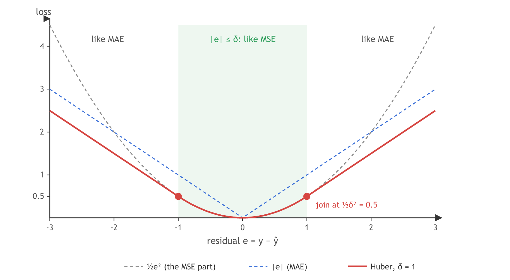
Huber loss uses the MSE shape for small errors and the MAE shape for large ones, with a hyperparameter δ (delta) for the switch:
δ is the error size where the loss stops being quadratic and becomes linear; it does not detect outliers by itself. Errors up to δ are treated like MSE, and errors beyond it grow in a straight line like MAE. The −½δ² makes the two pieces meet: at |e| = δ both give ½δ², and both have slope δ, so the curve has no kink. δ is tuned like any hyperparameter, by trying values on validation data.
Pseudo-Huber loss
The notes add a smooth version with no switch at all. It is close to a²/2 for small errors a and close to a straight line with slope δ for large ones:
Returning to the output's unit with RMSE
The notes add a fourth regression cost, the root mean squared error. MSE is in the output's unit squared (lakhs², cm²); the square root brings it back to the output's unit, while outliers still weigh heavily because the errors are squared first:
RMSE has its minimum at the same weights as MSE, so networks are trained on MSE and RMSE is reported as a metric.
Plotting L1 and L2 loss in the notebook
The materials' Loss function notebook calls MAE the L1 loss (least absolute deviations) and MSE the L2 loss (least squares). It draws both for guesses from −1 to 1 around a true value of 0, in TensorFlow 1:
x_guess = tf.lin_space(-1., 1., 100)
x_actual = tf.constant(0,dtype=tf.float32)

l1_loss = tf.abs((x_guess-x_actual))
l2_loss = tf.square((x_guess-x_actual))

with tf.Session() as sess:
    x_,l1_,l2_ = sess.run([x_guess, l1_loss, l2_loss])
    plt.plot(x_,l1_,label='l1_loss')
    plt.plot(x_,l2_,label='l2_loss')
    plt.legend()
    plt.show()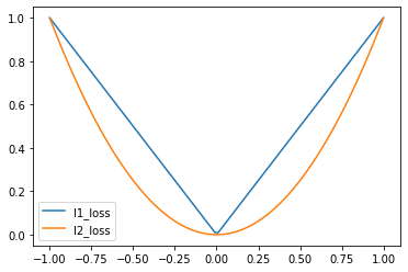
Output from the materials' notebook (TensorFlow 1.x, Python 3.7). TensorFlow 2 removed tf.lin_space and tf.Session; the same cells today:
import tensorflow as tf
import matplotlib.pyplot as plt

x_guess = tf.linspace(-1., 1., 100)            # was tf.lin_space
x_actual = tf.constant(0, dtype=tf.float32)
l1_loss = tf.abs(x_guess - x_actual)           # runs at once, no Session
l2_loss = tf.square(x_guess - x_actual)
plt.plot(x_guess, l1_loss, label='l1_loss')
plt.plot(x_guess, l2_loss, label='l2_loss')
plt.legend()
plt.show()
The notebook also makes the outlier point with numbers: the true value is 1, ten predictions are about 1, and one of them is 1000. The code below runs that case.
Computing the regression losses in NumPy
The loss functions
import numpy as np

def mse(y, y_hat):  return np.mean((y - y_hat) ** 2)
def mae(y, y_hat):  return np.mean(np.abs(y - y_hat))
def rmse(y, y_hat): return np.sqrt(mse(y, y_hat))

def huber(y, y_hat, delta=1.0):
    e = np.abs(y - y_hat)
    return np.mean(np.where(e <= delta, 0.5 * e ** 2, delta * e - 0.5 * delta ** 2))

def pseudo_huber(y, y_hat, delta=1.0):
    a = y - y_hat
    return np.mean(delta ** 2 * (np.sqrt(1 + (a / delta) ** 2) - 1))
The notebook's one prediction of 1000
y_true = np.ones(10)                      # the true value is 1
y_pred = np.array([1.1, 0.9, 1.0, 1.2, 0.8, 1.0, 0.9, 1.1, 1.0, 1000.0])

for name, fn in [("MSE", mse), ("MAE", mae), ("RMSE", rmse), ("Huber", huber)]:
    print(f"{name:5s} all 10: {fn(y_true, y_pred):10.3f}   without the 1000: {fn(y_true[:9], y_pred[:9]):.3f}")

print("pseudo-Huber at a = 1:", round(pseudo_huber(1.0, 0.0, delta=5), 3), round(pseudo_huber(1.0, 0.0, delta=0.25), 3))MSE all 10: 99800.112 without the 1000: 0.013 MAE all 10: 99.980 without the 1000: 0.089 RMSE all 10: 315.912 without the 1000: 0.115 Huber all 10: 99.856 without the 1000: 0.007 pseudo-Huber at a = 1: 0.495 0.195
The four curves for one residual
import matplotlib.pyplot as plt

e = np.linspace(-3, 3, 301)                    # residual y - ŷ
curves = {"L2: e²": e ** 2, "L1: |e|": np.abs(e),
          "Huber, δ = 1": np.array([huber(v, 0.0) for v in e]),
          "pseudo-Huber, δ = 1": np.array([pseudo_huber(v, 0.0) for v in e])}
for label, values in curves.items():
    plt.plot(e, values, label=label)
plt.ylim(0, 5); plt.xlabel("residual e = y - ŷ"); plt.ylabel("loss")
plt.title("Regression losses for one residual"); plt.legend(); plt.show()
print("at e = 3:", {k: round(float(v[-1]), 3) for k, v in curves.items()})at e = 3: {'L2: e²': 9.0, 'L1: |e|': 3.0, 'Huber, δ = 1': 2.5, 'pseudo-Huber, δ = 1': 2.162}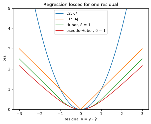
Fitting a line by gradient descent
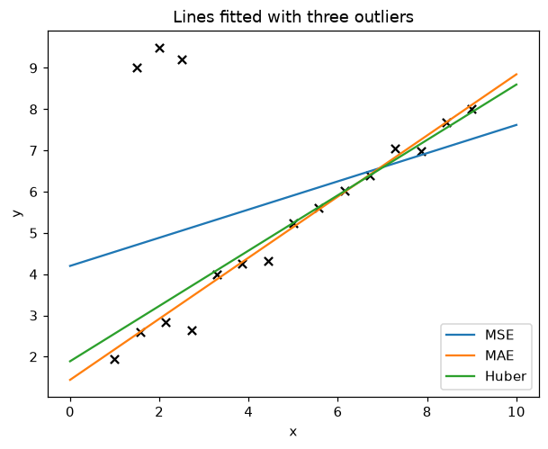
The board's picture of a line dragged by outliers can be rebuilt. Fifteen points follow a trend, three outliers sit top left, and the same gradient descent loop fits a line with each loss. Only the per-record slope g changes: the error itself for MSE (the ½ form), its sign for MAE (the sub-gradient), and the error clipped to [−1, 1] for Huber with δ = 1.
rng = np.random.default_rng(1)
x = np.linspace(1, 9, 15)
y = 0.8 * x + 1 + rng.normal(0, 0.4, size=15)   # points along a trend
x_out = np.append(x, [1.5, 2.0, 2.5])            # three outliers, top left
y_out = np.append(y, [9.0, 9.5, 9.2])

def fit(x, y, grad, steps=20000, lr=0.01):
    w, b = 0.0, 0.0
    for _ in range(steps):
        g = grad(y - (w * x + b))                # slope of the loss, per record
        w += lr * np.mean(g * x)
        b += lr * np.mean(g)
return w, bgrads = {"MSE": lambda e: e, "MAE": np.sign, "Huber": lambda e: np.clip(e, -1, 1)}
w0, b0 = fit(x, y, grads["MSE"])
print(f"no outliers, MSE : slope {w0:.3f}, intercept {b0:.3f}")
for name, g in grads.items():
w, b = fit(x_out, y_out, g)
print(f"with outliers, {name:5s}: slope {w:.3f}, intercept {b:.3f}")
plt.plot([0, 10], [b, w * 10 + b], label=name)
plt.scatter(x_out, y_out, color="black", marker="x")
plt.xlabel("x"); plt.ylabel("y"); plt.title("Lines fitted with three outliers"); plt.legend(); plt.show()no outliers, MSE : slope 0.771, intercept 1.184 with outliers, MSE : slope 0.342, intercept 4.199 with outliers, MAE : slope 0.741, intercept 1.437 with outliers, Huber: slope 0.671, intercept 1.888
What the losses printed
- One prediction of 1000 takes over MSE: 99800.112 with it, 0.013 without it. The outlier's squared error, 999², is more than 99.99% of the sum, which is the notebook's "the loss value is mainly dominated by 1000".
- MAE and Huber rise far less: MAE goes from 0.089 to 99.98, Huber from 0.007 to 99.856, because both grow in a straight line for a large error. RMSE (315.912) is back in the output's unit but still driven by the square.
- Pseudo-Huber matches the notebook's curves: 0.495 for δ = 5 and 0.195 for δ = 0.25 at an error of 1. A large δ keeps more of the quadratic shape.
- At e = 3 the curves print 9.0 for L2, 3.0 for L1, 2.5 for Huber (3 − ½) and 2.162 for pseudo-Huber.
- The fitted lines: without outliers MSE finds slope 0.771 and intercept 1.184. With the three outliers the MSE slope falls to 0.342 and the intercept jumps to 4.199, the swing on the board. MAE keeps 0.741 and 1.437, Huber 0.671 and 1.888.
Computing the losses in Keras
Keras has a class for each loss. Each call averages over the batch, and Keras's MSE has no ½, so on these three records the calls return the same values as the NumPy functions above: about 3.007 for MSE, 1.067 for MAE and 0.837 for Huber. In a model the loss goes in compile:
import keras

y_true = [[1.0], [1.0], [1.0]]
y_pred = [[1.1], [0.9], [4.0]]                 # errors 0.1, 0.1 and 3
print(keras.losses.MeanSquaredError()(y_true, y_pred))
print(keras.losses.MeanAbsoluteError()(y_true, y_pred))
print(keras.losses.Huber(delta=1.0)(y_true, y_pred))

# in a model: the loss by name, RMSE reported as a metric
model.compile(optimizer="adam", loss="huber",
              metrics=[keras.metrics.RootMeanSquaredError()])
MSE vs MAE vs Huber loss
| MSE (L2) | MAE (L1) | Huber | |
|---|---|---|---|
| Loss of one record | (y − ŷ)² | |y − ŷ| | ½e² up to δ, then δ|e| − ½δ² |
| Large errors | weigh heavily (squared) | weigh in proportion | weigh in proportion |
| Slope at the minimum | smooth, shrinks to 0 | sharp corner, sub-gradient | smooth |
| Extra setting | none | none | δ |
| Keras name | "mse" | "mae" | "huber" |
Where you use MSE, MAE and Huber loss
- MSE for clean regression targets such as a salary or a house price with no wild rows: it is smooth and trains fast.
- MAE when some targets are wrong or extreme, such as sensor readings with spikes, and the line should follow the bulk of the data.
- Huber when you want both: smooth training near the minimum and limited pull from outliers. It is common in reinforcement learning, where target values can jump.
Related
- Previous: Loss and cost functions
- Next: Binary cross-entropy
- Refresher: MSE, MAE and RMSE in the Machine Learning course
- Reference: Regression losses in the Keras documentation
- Set
delta=0.1in the fit's Huber slope (np.clip(e, -0.1, 0.1)): Huber then behaves almost like MAE: the slope becomes 0.730, next to MAE's 0.741. - Put 2.0 in place of the 1000: MSE prints 0.112 and MAE 0.18, because no error is large enough for the square to take over.
- Move the three outliers to the top right (
x_outends 8.5, 9, 9.5 andy_outends 14, 14.5, 15): the MSE slope jumps to about 1.255 while MAE stays near 0.805.
Little by little, you're building something great.