ReLU and its variants
ReLU (rectified linear unit) is an activation function that outputs max(0, z): the input itself when it is positive and 0 when it is negative.
Last updated: 05 Oct, 2026 · NumPy
The Activation functions lesson showed that sigmoid and tanh both saturate, so a deep network's gradient still vanishes. ReLU is the next answer, and today it is the most popular activation function in hidden layers.
Computing ReLU and its derivative
A negative input becomes 0 and a positive one passes through unchanged: the video's examples are 1 → 1, 2 → 2 and 3 → 3. The derivative is either 0 or 1. At exactly z = 0 the derivative is not defined; code takes 0 or 1 there (the notebook calls this a sub-gradient), and it rarely matters because z is almost never exactly 0.
Deriving the dead neuron
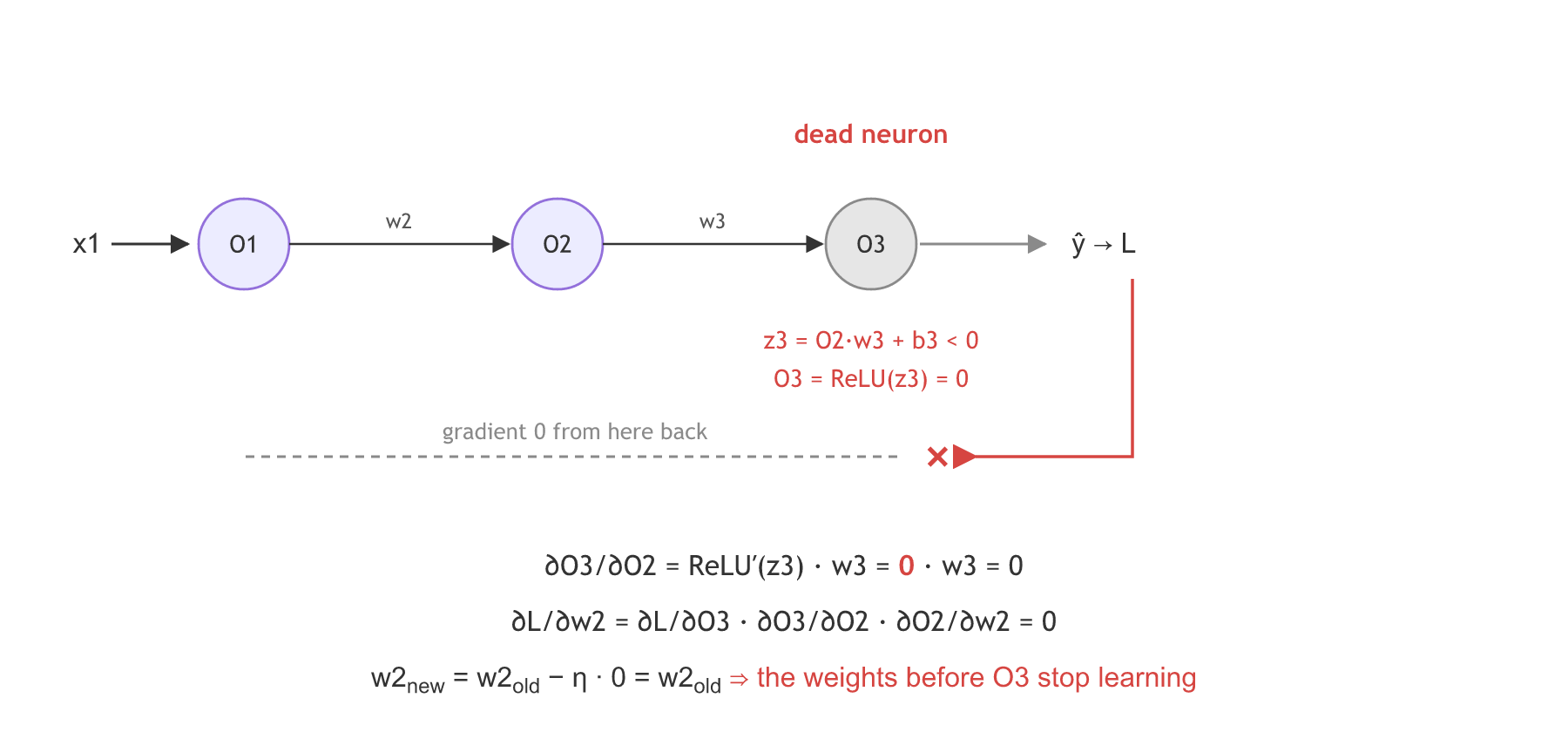
A derivative of 1 is good news: the gradient passes through without shrinking, so ReLU does not cause vanishing gradients for positive inputs. A derivative of 0 is the problem. The notes write the chain for the network x1 → O1 → O2 → O3 → loss, where O3 = ReLU(z3) with z3 = O2·w3 + b3:
If z3 is negative, ReLU′(z3) = 0, so the whole chain is 0 and w2_new = w2_old − η · 0 = w2_old. The weights behind that neuron get no update. If z3 is negative for every record, the neuron outputs 0 for all of them and never recovers: a dead neuron, also called the dead ReLU problem. The video says the neuron dies when "one of the weights" becomes zero; it is the derivative that is 0, because the neuron's z is negative.
Weighing ReLU's advantages
- No exponential: max(0, z) is a comparison, much quicker than sigmoid or tanh.
- No saturation for positive inputs: the derivative is 1, so gradients do not vanish there.
- Not zero centred: it passes through 0 but never outputs a negative value. The video says ReLU also solves tanh's problem and then, a moment later, that it is not zero centric; the second is right.
- Dead neurons: a negative input gives a derivative of 0, the disadvantage above.
Fixing dead neurons with Leaky ReLU
Leaky ReLU keeps a small slope α for negative inputs instead of 0, so the output for z < 0 is a small negative number and the derivative is α, never 0:
The video uses α = 0.01, f(z) = max(0.01z, z). The notes treat α as a hyperparameter you pick, with 0.01, 0.02 and 0.03 as values to try.
The run below makes the dead neuron happen. One neuron starts with bias −3, so z < 0 for every record. It trains for 500 steps on a target it could fit, once with ReLU (α = 0) and once with Leaky ReLU (α = 0.01):
import numpy as np
rng = np.random.default_rng(1)
X = rng.uniform(0, 1, (50, 2))                # 50 records, 2 inputs between 0 and 1
y = X @ np.array([2.0, -1.0]) + 0.5           # the target the neuron should learn

def train(alpha, steps=500, eta=0.5):
    w, b = np.array([0.5, 0.5]), -3.0         # bias -3: z < 0 for every record
    for _ in range(steps):
        z = X @ w + b
        out = np.where(z > 0, z, alpha * z)   # ReLU when alpha = 0
        g = (out - y) * np.where(z > 0, 1.0, alpha)   # dL/dz, through the derivative
        w = w - eta * (X.T @ g) / len(y)
        b = b - eta * g.mean()
    return w, b

for alpha in [0.0, 0.01]:
    w, b = train(alpha)
print(f"alpha = {alpha}: w = {np.round(w, 3)}, b = {b:.3f}")alpha = 0.0: w = [0.5 0.5], b = -3.000 alpha = 0.01: w = [ 2.003 -1. ], b = 0.498
- With ReLU, w and b never move: w stays [0.5, 0.5] and b stays −3.0 after 500 steps. Every gradient is 0, so this neuron is dead.
- With Leaky ReLU they learn: the 0.01 slope lets a small gradient through, b climbs past 0, and the weights reach about [2.003, −1.0] with b = 0.498, close to the target's 2, −1 and 0.5.
Weighing Leaky ReLU against ReLU
The notebook then makes two points about Leaky ReLU. The slope does not have to be 0.01: a parameter-based method lets it take other values, or learn it, which is where PReLU below comes from. And a caution: in theory Leaky ReLU has all of ReLU's advantages and no dead neurons, but in practice it has not been fully proved that Leaky ReLU is always better than ReLU.
Smoothing the corner with ELU
ELU (exponential linear unit) replaces the negative side with an exponential curve that flattens out at −α:
It has no dead ReLU issue, its negative outputs pull the mean output close to 0 (close to zero centred), and its cost is the exponential, so it is slightly more expensive to compute. With α = 1, the plotted case, the derivative runs from 0 to 1.
Learning the slope with PReLU
Parametric ReLU (PReLU) is Leaky ReLU's shape with the slope for negative inputs turned into a parameter the network learns in backpropagation, one aᵢ per neuron:
- aᵢ = 0 gives ReLU.
- aᵢ a small fixed number (such as 0.01) gives Leaky ReLU.
- aᵢ learnable gives PReLU.
The video reads the condition as "w of i greater than zero"; the variable in the condition is the input zᵢ, and aᵢ is the slope.
Using Swish, the self-gated function
Swish multiplies the input by its own sigmoid, so the sigmoid acts as a gate on the value:
For large positive z it behaves like ReLU, and for negative z it dips a little below 0 before returning to 0. The video says Swish has one problem, that its derivative at zero cannot be found. That is the case for ReLU, not Swish: Swish is smooth everywhere, and its derivative at 0 is σ(0) = 0.5.
Computing the ReLU family in NumPy
ReLU and Leaky ReLU
import numpy as np

def sigmoid(z):
    return 1 / (1 + np.exp(-z))

def relu(z):
    return np.maximum(0, z)

def leaky_relu(z, alpha=0.01):
    return np.where(z > 0, z, alpha * z)
ELU and Swish
def elu(z, alpha=1.0):
    return np.where(z > 0, z, alpha * (np.exp(z) - 1))

def swish(z):
    return z * sigmoid(z)                     # x times sigmoid(x), smooth everywhere
Their derivatives
def d_relu(z):
    return np.where(z > 0, 1.0, 0.0)          # 0 for z < 0, 1 for z > 0

def d_leaky(z, alpha=0.01):
    return np.where(z > 0, 1.0, alpha)

def d_elu(z, alpha=1.0):
    return np.where(z > 0, 1.0, alpha * np.exp(z))

def d_swish(z):
    s = sigmoid(z)
return s + z * s * (1 - s)z = np.array([-2.0, -0.5, 0.0, 0.5, 2.0])
print("z ", z)
print("relu ", relu(z), " derivative", d_relu(z))
print("leaky 0.01 ", leaky_relu(z), " derivative", d_leaky(z))
print("elu ", np.round(elu(z), 4), " derivative", np.round(d_elu(z), 4))
print("swish ", np.round(swish(z), 4), " derivative", np.round(d_swish(z), 4))
print("relu on 1, 2, 3:", relu(np.array([1, 2, 3])))z [-2. -0.5 0. 0.5 2. ] relu [0. 0. 0. 0.5 2. ] derivative [0. 0. 0. 1. 1.] leaky 0.01 [-0.02 -0.005 0. 0.5 2. ] derivative [0.01 0.01 0.01 1. 1. ] elu [-0.8647 -0.3935 0. 0.5 2. ] derivative [0.1353 0.6065 1. 1. 1. ] swish [-0.2384 -0.1888 0. 0.3112 1.7616] derivative [-0.0908 0.26 0.5 0.74 1.0908] relu on 1, 2, 3: [1 2 3]
What the values show
- ReLU turns −2 and −0.5 into 0 and keeps 0.5 and 2; its derivative is 0 or 1 (0 at z = 0 in this code).
- Leaky ReLU keeps −0.02 and −0.005, and its derivative on the negative side is 0.01, never 0.
- ELU gives −0.8647 at z = −2, heading for −1, with derivative 0.1353 = e^(−2).
- Swish gives −0.2384 at z = −2, and its derivative at 0 is 0.5: defined and smooth.
Plotting the ReLU family and its derivatives
The same four functions on one figure, the function on top and its derivative below. Leaky ReLU is drawn with α = 0.1 because a 0.01 slope looks flat at this scale.
import matplotlib.pyplot as plt

z = np.linspace(-5, 5, 501)
rows = [("ReLU", relu, d_relu), ("Leaky ReLU, α = 0.1", lambda v: leaky_relu(v, 0.1), lambda v: d_leaky(v, 0.1)),
        ("ELU, α = 1", elu, d_elu), ("Swish", swish, d_swish)]
fig, axes = plt.subplots(2, 4, figsize=(12, 5))
for col, (name, f, df) in enumerate(rows):
    axes[0, col].plot(z, f(z))
    axes[0, col].set_title(name)
    axes[1, col].plot(z, df(z), c="tab:orange")
    axes[1, col].set_title("derivative")
    axes[1, col].set_ylim(-0.2, 1.2)
    for ax in axes[:, col]:
        ax.axhline(0, c="grey", lw=0.6)
        ax.axvline(0, c="grey", lw=0.6)
plt.tight_layout()
plt.show()
i = np.argmin(swish(z))
print(f"swish minimum: {swish(z)[i]:.4f} at z = {z[i]:.2f}")swish minimum: -0.2785 at z = -1.28
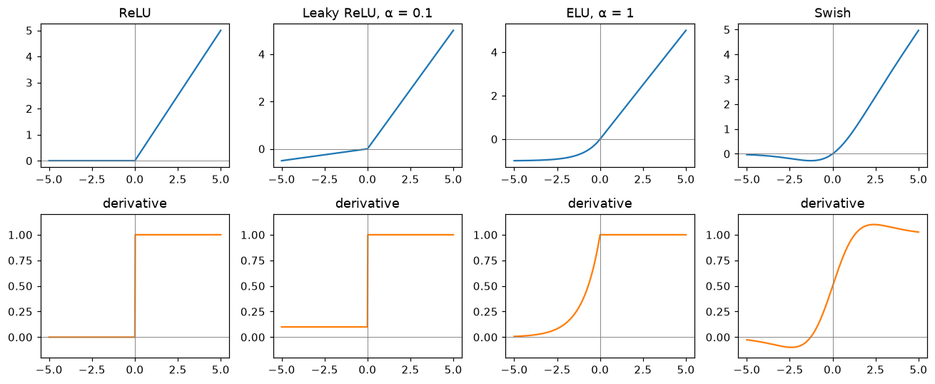
Swish's lowest value is −0.2785 at z = −1.28, the dip below 0. ReLU and Leaky ReLU have a corner at 0, where the derivative jumps; ELU and Swish have none.
In Keras each of these is one argument or one layer. Set Leaky ReLU's slope yourself, because Keras's default is not the video's 0.01:
from keras import layers

layers.Dense(8, activation="relu")            # ReLU
layers.Dense(8, activation="elu")             # ELU, alpha = 1
layers.Dense(8, activation="swish")           # Swish (Keras also calls it silu)
layers.LeakyReLU(negative_slope=0.01)         # Leaky ReLU with the video's 0.01
layers.PReLU()                                # PReLU: the slope is learned
ReLU vs Leaky ReLU vs PReLU vs ELU vs Swish
| For z < 0 | Derivative for z < 0 | Dead neurons | Cost | |
|---|---|---|---|---|
| ReLU | 0 | 0 | yes | cheapest |
| Leaky ReLU | αz, α = 0.01 | α | no | cheap |
| PReLU | aᵢz, aᵢ learned | aᵢ | no | cheap, one extra parameter per neuron |
| ELU | α(e^z − 1) | αe^z | no | an exponential |
| Swish | zσ(z), dips to −0.28 | smooth, small | no | an exponential |
Where you use ReLU and its variants
- Hidden layers by default: ReLU is the first choice for the hidden layers of a deep network.
- When training stalls: if many neurons output 0 for every record, switch to Leaky ReLU, PReLU or ELU.
- Deeper modern networks: Swish (Keras's "swish" or "silu") appears in many large image and language models.
Related
- Previous: Activation functions
- Next: Softmax
- In the dead-neuron run, change the starting bias to
-0.2. Does plain ReLU learn now? - Train with
alpha = 0.1andsteps=100. Does a larger slope revive the neuron faster? - Print
d_swish(np.array([-1.28])). Why is it close to 0 at Swish's lowest point?
You understood something today that you didn't yesterday.