Building an ANN in Keras
An ANN in Keras is a Sequential model: a stack of Dense layers, each with a number of neurons and an activation function, compiled with an optimizer, a loss function and a metric before it trains.
Last updated: 05 Oct, 2026 · TensorFlow 2 / Keras
Preparing the churn data left 8,000 scaled training rows with 11 features each. This lesson builds the network that learns from them, the same network the theory lessons drew by hand.
Importing TensorFlow and Keras
The video uses TensorFlow, a deep learning library open-sourced by Google; PyTorch, from Facebook (now Meta), can do the same things. Before TensorFlow 2.0, Keras was a separate library, a wrapper that called TensorFlow's functions through simple ones, and the two had to be installed separately with matching versions. From TensorFlow 2.0, Keras ships inside TensorFlow as tensorflow.keras.
The video credits the DeepMind team with creating TensorFlow; it was built by the Google Brain team. And since TensorFlow 2.16, pip install tensorflow brings Keras 3, a separate package that runs on TensorFlow, JAX or PyTorch; tensorflow.keras points to it, so the imports below still work.
## Part 2 Now lets create the ANN
from tensorflow.keras.models import Sequential
from tensorflow.keras.layers import Dense
from tensorflow.keras.layers import LeakyReLU,PReLU,ELU,ReLU
from tensorflow.keras.layers import Dropout
Sequential holds the model, Dense makes a layer of neurons and Dropout is the layer from Dropout. LeakyReLU, PReLU, ELU and ReLU are activation layers from ReLU and its variants; the video imports them to show they exist but uses the activation names as strings instead.
Reading Sequential, Dense and activation
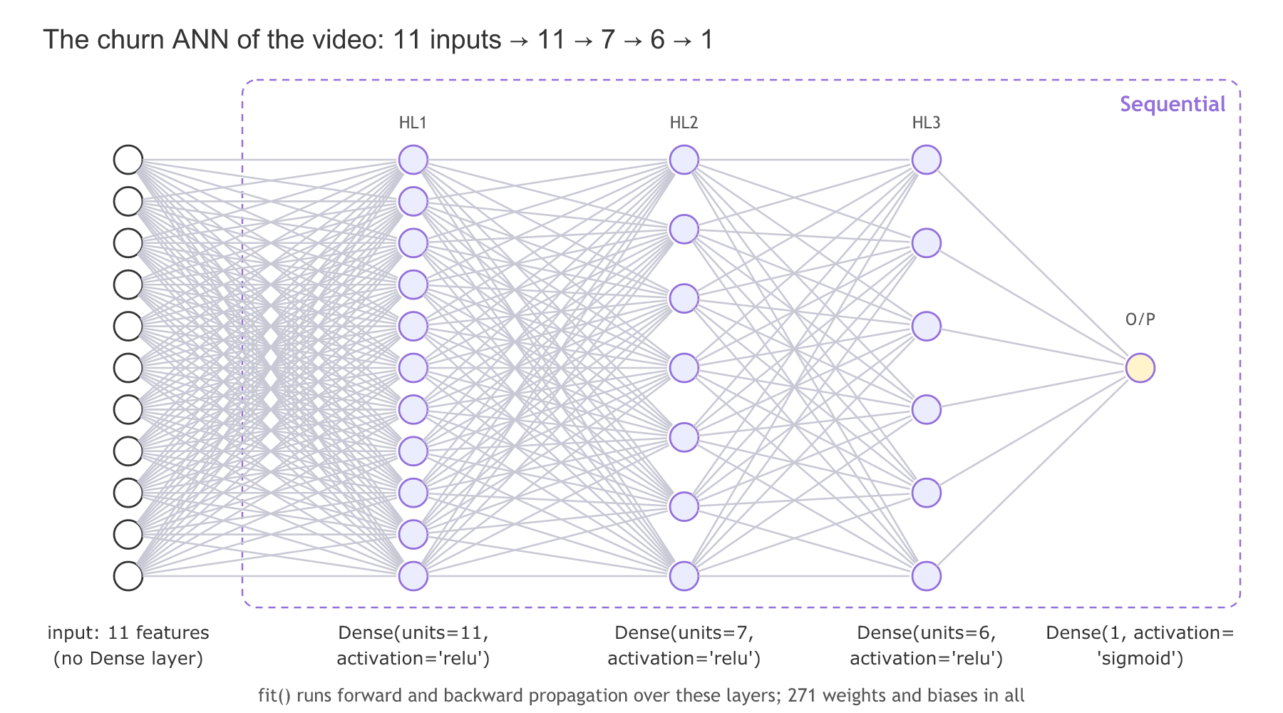
On the board, the network has 11 inputs, one per feature, hidden layers whose neurons connect to every neuron of the next layer, and a single output neuron, enough for a binary answer of 1 or 0.
- Sequential is the whole network taken as one block: layers stacked in order, each feeding the next. The video says Sequential does the forward and backward propagation. It only holds the layers;
compile()andfit()run the training. - Dense creates the circles: a layer of neurons, each connected to all outputs of the layer before. Hidden layers and the output layer are Dense layers.
- The activation is chosen per layer: ReLU, PReLU, sigmoid or tanh, as in Choosing an activation function.
Adding the Dense layers
classifier=Sequential() starts an empty network, and each classifier.add(Dense(...)) adds a layer with units neurons. The video counts 11 inputs in X_train, adds Dense(units=11, activation='relu'), then hidden layers of 7 and 6 ReLU neurons ("six or seven, whatever you want"), and an output layer of one neuron. For a binary classification the output activation is sigmoid, which turns the last neuron's value into a probability between 0 and 1.
### Lets initialize the ANN
classifier=Sequential()
## Adding the input Layer
classifier.add(Dense(units=11,activation='relu'))
# adding the first hidden layer
classifier.add(Dense(units=7,activation='relu'))
##adding the second hidden layer
classifier.add(Dense(units=6,activation='relu'))
##  Adding the output layer
classifier.add(Dense(1,activation='sigmoid'))
The comment calls Dense(units=11) the input layer, and the video says its ReLU applies to the next layer. In Keras the input layer is not a Dense layer: the 11 features of X_train are the inputs, and Dense(units=11) is the first hidden layer, which happens to have 11 neurons. A layer's activation acts on that same layer's outputs. So the network is 11 inputs → 11 → 7 → 6 → 1, three hidden layers and an output. How many neurons each layer should have is the subject of Hidden layers and neurons with Keras Tuner.
Counting the weights of the network
Each Dense layer holds a kernel, one weight per input and neuron, and one bias per neuron, so it has inputs × units + units parameters. The video's classifier.get_weights() later prints exactly these arrays: an 11-value bias after the first kernel, then an 11 × 7 kernel.
params = n_in * n_out + n_out # kernel (n_in, n_out) + bias (n_out,)sizes = [11, 11, 7, 6, 1] # 11 inputs, then the units of each Dense layer
total = 0
for n_in, n_out in zip(sizes, sizes[1:]):
params = n_in * n_out + n_out # kernel weights + one bias per neuron
total += params
print(f"Dense({n_out}): kernel ({n_in}, {n_out}) + bias ({n_out},) = {params} parameters")
print("total:", total)
sizes_2024 = [12, 64, 32, 1] # the 2024 version: 12 inputs, 64, 32, 1
print("2024 model:", [i * o + o for i, o in zip(sizes_2024, sizes_2024[1:])],
sum(i * o + o for i, o in zip(sizes_2024, sizes_2024[1:])))Dense(11): kernel (11, 11) + bias (11,) = 132 parameters Dense(7): kernel (11, 7) + bias (7,) = 84 parameters Dense(6): kernel (7, 6) + bias (6,) = 48 parameters Dense(1): kernel (6, 1) + bias (1,) = 7 parameters total: 271 2024 model: [832, 2080, 33] 2945
- 132 + 84 + 48 + 7 = 271 parameters in the video's network. Training adjusts all 271 together, which is why the video says to imagine how many weights are being trained in parallel.
- The 2024 version of this practical has 12 inputs and layers of 64, 32 and 1: 832 + 2080 + 33 = 2945 parameters, the numbers its
model.summary()prints below.
Running the untrained network forward
Before training, the network is the forward propagation of Forward propagation with random weights. The NumPy version below starts the kernels the way Dense does (Glorot uniform, zero biases) and pushes five test customers through the four layers.
import numpy as np

rng = np.random.default_rng(0)
def glorot_uniform(n_in, n_out):           # the Dense default
    limit = np.sqrt(6 / (n_in + n_out))
    return rng.uniform(-limit, limit, (n_in, n_out))

sizes = [11, 11, 7, 6, 1]
a = X_test[:5]                             # five scaled test customers
for n_in, n_out in zip(sizes, sizes[1:]):
    z = a @ glorot_uniform(n_in, n_out) + np.zeros(n_out)   # zero biases
    a = 1 / (1 + np.exp(-z)) if n_out == 1 else np.maximum(0, z)
    print(f"after Dense({n_out}): shape {a.shape}")
print("untrained churn probabilities:", a.ravel().round(3))
print("true labels:", y_test[:5].tolist())after Dense(11): shape (5, 11) after Dense(7): shape (5, 7) after Dense(6): shape (5, 6) after Dense(1): shape (5, 1) untrained churn probabilities: [0.711 0.546 0.523 0.43 0.462] true labels: [0, 1, 0, 0, 0]
- The shapes go (5, 11) → (5, 7) → (5, 6) → (5, 1): five customers, one column per neuron of each layer.
- The untrained probabilities fall between 0.43 and 0.71 with no link to the true labels (the highest, 0.711, is for a customer who stayed), because the random weights know nothing yet. Training moves them towards 0 for customers who stay and 1 for those who leave.
Compiling with Adam and binary cross-entropy
compile() fixes how the network will learn: the Adam optimizer, the Binary cross-entropy loss for a yes/no output, and accuracy as the metric to print.
classifier.compile(optimizer='adam',loss='binary_crossentropy',metrics=['accuracy'])To set the learning rate, the video creates an Adam optimizer object and passes it to compile as optimizer=opt. Create opt first, then compile with it.
import tensorflow
opt=tensorflow.keras.optimizers.Adam(learning_rate=0.01)
The video says Adam's default learning rate is 0.01. The default is 0.001, so learning_rate=0.01 makes the video's run take steps ten times larger than the default.
Building the 2024 version of the model
The 2024 ANN-CLassification-Churn notebook builds the same kind of network in one call, passing the layers as a list. It keeps all three Geography columns, so X_train has 12 features, and it names the input size on the first layer with input_shape.
## Build Our ANN Model
model=Sequential([
    Dense(64,activation='relu',input_shape=(X_train.shape[1],)), ## HL1 Connected wwith input layer
    Dense(32,activation='relu'), ## HL2
    Dense(1,activation='sigmoid')  ## output layer
]

)model.summary()Model: "sequential_1"
_________________________________________________________________
Layer (type) Output Shape Param #
=================================================================
dense_3 (Dense) (None, 64) 832
dense_4 (Dense) (None, 32) 2080
dense_5 (Dense) (None, 1) 33
=================================================================
Total params: 2945 (11.50 KB)
Trainable params: 2945 (11.50 KB)
Non-trainable params: 0 (0.00 Byte)
_________________________________________________________________(None, 64) means any number of rows and 64 outputs. The model is sequential_1 with layers dense_3 to dense_5 because a model had already been built earlier in the same session. On Keras 3, input_shape= on a layer prints a warning that asks for an Input object as the first layer instead:
from tensorflow.keras import Input

model = Sequential([
    Input(shape=(12,)),                 # the 12 features, no Dense layer
    Dense(64, activation='relu'),
    Dense(32, activation='relu'),
    Dense(1, activation='sigmoid'),
])
The 2022 network vs the 2024 network
| The video (2022) | ANN-CLassification-Churn (2024) | |
|---|---|---|
| Features | 11 (drop_first=True) | 12 (all three countries) |
| Hidden layers | 11, 7, 6 (ReLU) | 64, 32 (ReLU) |
| Output | Dense(1, sigmoid) | Dense(1, sigmoid) |
| Parameters | 271 | 2945 |
| Optimizer | Adam, learning_rate=0.01 | Adam, learning_rate=0.01 |
| Built with | classifier.add(...) per layer | a list passed to Sequential |
Where you use a Sequential model
- Tabular classification and regression, like churn, credit risk or house prices: a few Dense layers are often enough.
- Any network that is one straight stack of layers, including the CNN in CNN in Keras.
- Prototyping before tuning the sizes with Keras Tuner.
classifier.add(...) cells a second time adds the layers again to the same model, so the network quietly grows. Re-run classifier=Sequential() before adding layers again, or build the model in one cell as the 2024 version does.Related
- Previous: Preparing the churn data
- Next: Training and evaluating an ANN
- See also: Forward propagation, Weight initialization
- Reference: Dense layer in the Keras API
- Change
sizesto[11, 6, 1], the earlier Untitled63 network with one hidden layer of 6, and count its parameters. - In the forward pass, replace the ReLU with
np.tanh(z)and compare the untrained probabilities. - Add a fourth Dense layer of 4 units to
sizesand check which layer's parameter count changes.
This is what real progress feels like.