Adagrad
Adagrad (adaptive gradient descent) is an optimizer that divides the learning rate by the square root of the running sum of squared gradients, so the step size of each weight shrinks as training goes on.
Last updated: 05 Oct, 2026 · TensorFlow 2 / Keras
In gradient descent, SGD, mini-batch SGD and SGD with momentum, the learning rate η is fixed. The video asks for something better: a high learning rate while the weights are far from the global minima, and a smaller one as they get close. A learning rate that changes by itself is adaptive.
Replacing the learning rate with η′
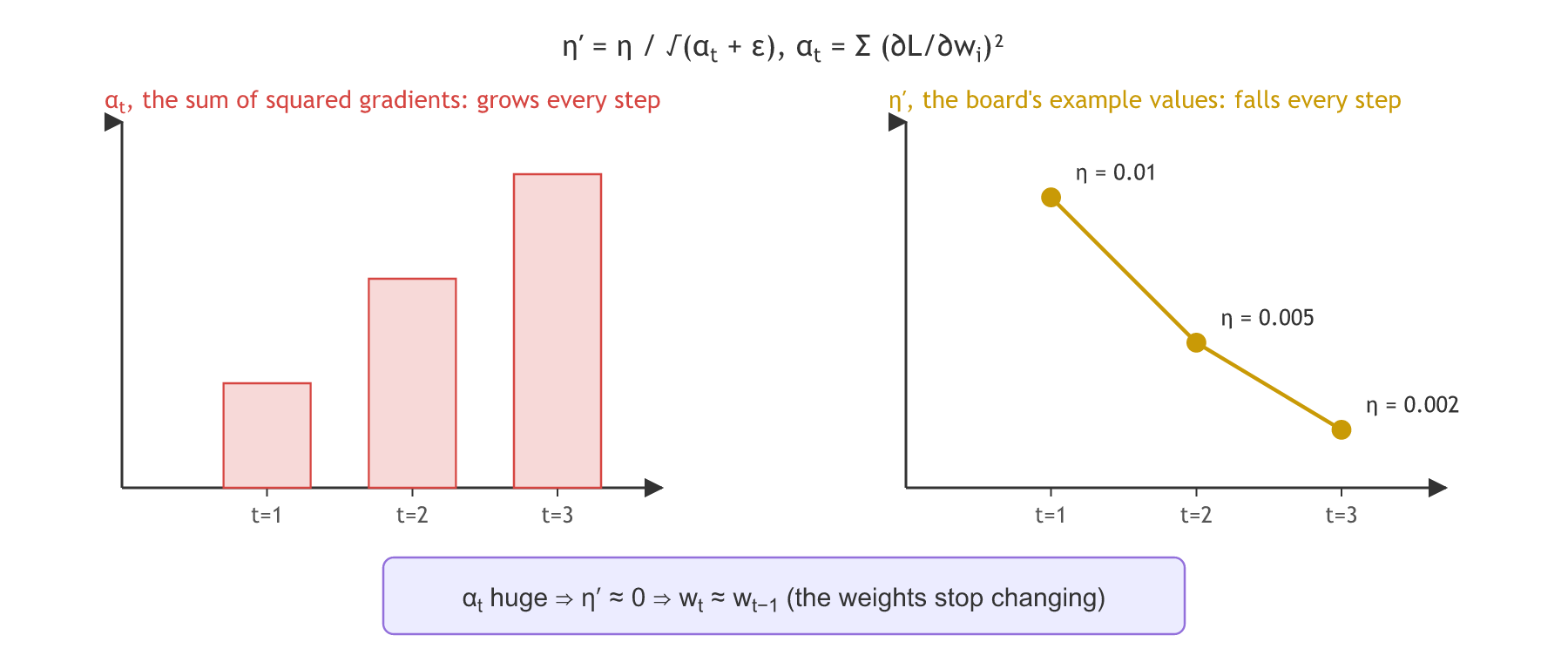
Adagrad keeps the weight update and replaces η with a new value η′ (eta prime):
- ε (epsilon) is a small number that avoids dividing by 0 when αt is still 0.
- αt adds up the square of the gradient at every step from 1 to t, so it can only grow.
- Because αt is in the denominator, a growing αt makes η′ smaller at every step: the learning rate decreases on its way to the global minima.
Three small slips in the clip: the video says "summation of all the previous weights", but αt sums the squared gradients; it says "focus on the numerator" for αt, which sits in the denominator; and the board indexes the sum with t, where it should be i. The board's example values are η = 0.01 at t = 1, 0.005 at t = 2 and 0.002 at t = 3. The video says "0.05" for t = 2, but the value must fall, and the board writes 0.005.
The formula on the board puts ε inside the square root, and so does Keras. The original paper and PyTorch write η/(√αt + ε) instead; with ε this small, the two give the same steps.
Why Adagrad stops learning
The same sum is Adagrad's weakness, which the video takes up at the start of the next lesson. In a deep network the sum keeps growing for thousands of steps and becomes a huge number. Then η′ is close to 0, and the update barely moves the weight:
Running Adagrad in NumPy
The Adagrad loop
The update is four lines inside a loop. gradient is the derivative of whatever loss is being trained.
alpha_t = 0.0
for t in range(1, steps + 1):
    g = gradient(w)
    alpha_t += g ** 2                         # α_t = Σ (∂L/∂w)² over every step so far
    lr_t = lr / np.sqrt(alpha_t + eps)        # η′ = η / √(α_t + ε)
    w = w - lr_t * g
The first three learning rates
A loss of w²/2 starting from w = 1, with the board's η = 0.01. The gradient of w²/2 is w, so the first gradient is 1 and η′ at t = 1 is exactly 0.01:
import numpy as np

lr, eps, w, alpha_t = 0.01, 1e-8, 1.0, 0.0
for t in range(1, 4):
    g = w                                     # the gradient of w²/2
    alpha_t += g ** 2
    lr_t = lr / np.sqrt(alpha_t + eps)
    w = w - lr_t * g
print(f"t = {t}: gradient {g:.4f} α_t {alpha_t:.4f} η′ = {lr_t:.5f} w = {w:.4f}")t = 1: gradient 1.0000 α_t 1.0000 η′ = 0.01000 w = 0.9900 t = 2: gradient 0.9900 α_t 1.9801 η′ = 0.00711 w = 0.9830 t = 3: gradient 0.9830 α_t 2.9463 η′ = 0.00583 w = 0.9772
The failure case on a far target
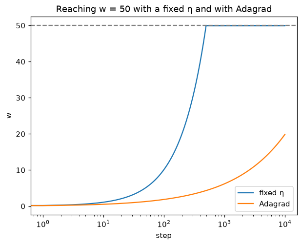
Now a target that is far away: an absolute error loss |w − 50| from w = 0, whose gradient is −1 until w reaches 50. A fixed learning rate of 0.1 walks there in about 500 steps. Adagrad starts with the same η = 0.1:
import matplotlib.pyplot as plt

def gradient(w):
    return np.sign(w - 50.0)                  # the slope of |w − 50|

for name in ("fixed η", "Adagrad"):
    w, alpha_t, reached, track = 0.0, 0.0, None, []
    for t in range(1, 10_001):
        g = gradient(w)
        alpha_t += g ** 2
        lr_t = 0.1 if name == "fixed η" else 0.1 / np.sqrt(alpha_t + 1e-8)
        w = w - lr_t * g
        track.append(w)
        if reached is None and w >= 49.5:
            reached = t
        if name == "Adagrad" and t in (1, 10, 100, 1000, 10_000):
            print(f"Adagrad step {t:>6}: η′ = {lr_t:.4f}  w = {w:.2f}")
    print(f"{name}: w after 10,000 steps = {w:.2f}, reached 50 at step {reached}")
    plt.plot(track, label=name)
plt.axhline(50, color="gray", ls="--"); plt.xscale("log")
plt.xlabel("step"); plt.ylabel("w"); plt.title("Reaching w = 50 with a fixed η and with Adagrad")
plt.legend(); plt.show()fixed η: w after 10,000 steps = 50.00, reached 50 at step 495 Adagrad step 1: η′ = 0.1000 w = 0.10 Adagrad step 10: η′ = 0.0316 w = 0.50 Adagrad step 100: η′ = 0.0100 w = 1.86 Adagrad step 1000: η′ = 0.0032 w = 6.18 Adagrad step 10000: η′ = 0.0010 w = 19.85 Adagrad: w after 10,000 steps = 19.85, reached 50 at step None
Reading the shrinking learning rate
- η′ falls 0.01, 0.0071, 0.0058 over the first three steps. The board's 0.01, 0.005, 0.002 show the same direction with made-up values; the real fall depends on the gradients.
- With a gradient of 1 at every step, αt = t, so η′ = 0.1/√t: 0.0316 at step 10, 0.01 at step 100, 0.001 at step 10,000.
- Adagrad never reaches 50. After 10,000 steps it is at about 20, while the fixed learning rate arrived around step 500. This is wt ≈ wt−1 from the board, in numbers.
Adagrad in Keras
import keras

opt = keras.optimizers.Adagrad(learning_rate=0.01, epsilon=1e-7)
model.compile(optimizer=opt, loss="mse")
Keras starts the running sum at a small positive value, initial_accumulator_value=0.1, rather than at 0, so the very first step is not divided by ε alone. Its default learning rate is 0.001; the code above sets 0.01, the board's value.
Fixed learning rate vs Adagrad
| Fixed learning rate (SGD, momentum) | Adagrad | |
|---|---|---|
| Learning rate | η, the same at every step | η′ = η/√(αt + ε), smaller at every step |
| Per weight | one η for all weights | each weight has its own αt and η′ |
| Far from the minimum | steps of the same size | big first steps, then ever smaller |
| Long training | keeps moving | can stall: η′ ≈ 0 and wt ≈ wt−1 |
Where you use Adagrad
- Sparse features, such as word counts: a rare feature's weight gets few gradients, so its αt stays small and its learning rate stays high, while common features slow down. The materials' optimizer notebook gives the GloVe word vectors as an example trained with Adagrad.
- Short trainings where the shrinking learning rate is an advantage rather than a stall.
- As a step towards RMSprop, which keeps the per-weight scaling and fixes the stall.
Related
- Previous: SGD with momentum
- Next: RMSprop and Adadelta
- In the first example start from
w = 5.0: the first gradient is 5, so η′ at t = 1 is 0.002, already far below η. - In the failure run change Adagrad's
0.1 / np.sqrt(...)to2.0 / np.sqrt(...): it now reaches 50, which shows the stall is about the fall of η′, not about the target. - Print
alpha_tat step 10,000 in the failure run: it is 10,000, one per step.
Slow is fine. Stopping is the only problem.