Gradient descent
Gradient descent is an optimisation algorithm that starts from one guess for the parameters and repeatedly steps them downhill along the slope of the cost function until the cost stops falling.
Last updated: 05 Oct, 2026 · scikit-learn 1.9.1
The Cost function lesson tried θ₁ = 1, 0.5 and 0 by hand. Gradient descent replaces the guessing: start at one point and let the slope say which way to move.
Repeating the update until convergence
Once you are at a point on the cost curve, keep updating θ₁ instead of trying new values. The convergence algorithm says: repeat until convergence, which works like a while loop, and in each pass update every θⱼ:
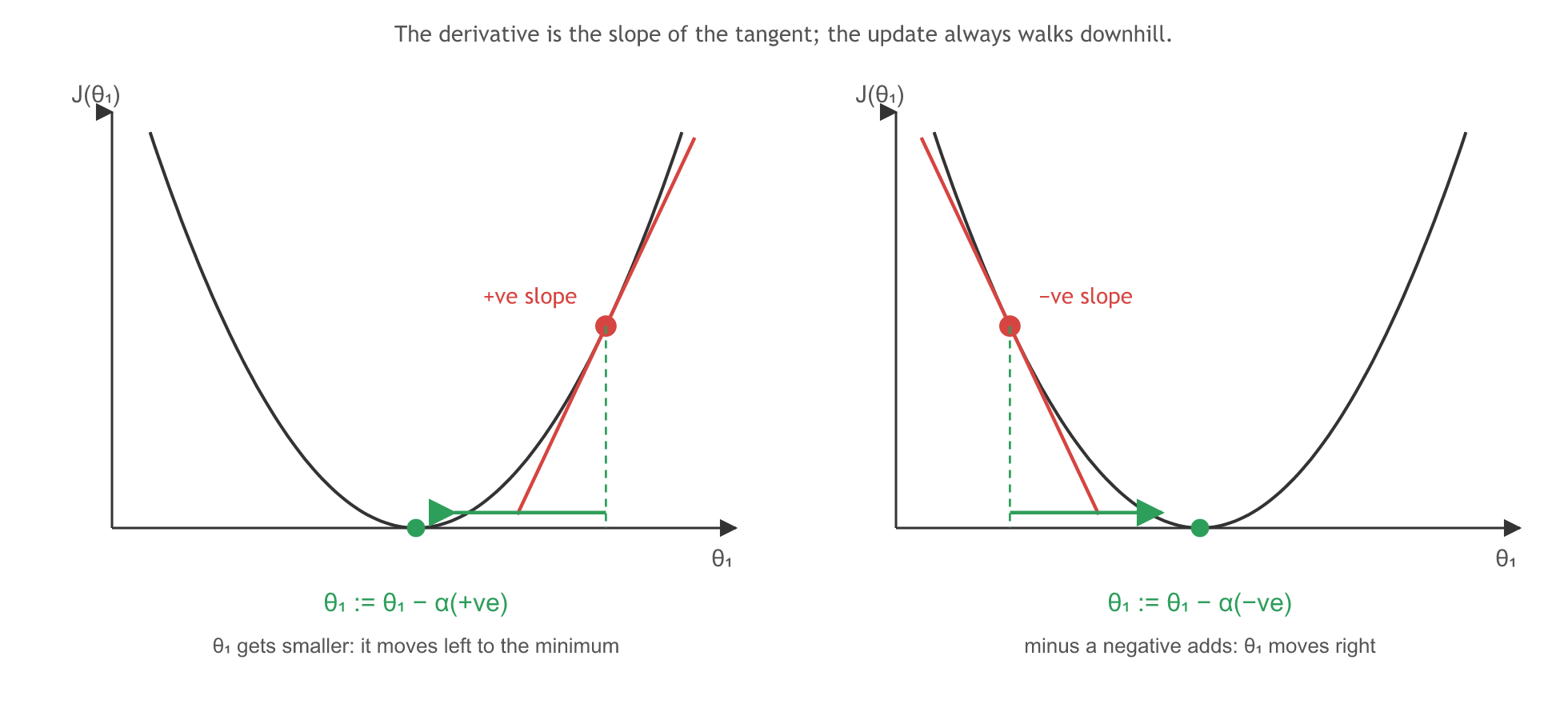
The derivative is the slope of the curve at the current point. Draw the tangent there: if its right end points upward, the slope is positive.
- Positive slope (a point on the right arm): θ₁ := θ₁ − α × (positive number), so θ₁ gets smaller and moves left, towards the global minimum.
- Negative slope (a point on the left arm): θ₁ := θ₁ − α × (negative number). Minus times minus is plus, so θ₁ gets bigger and moves right, again towards the minimum.
- Either way, after enough iterations θ₁ reaches the global minimum.
Choosing the learning rate
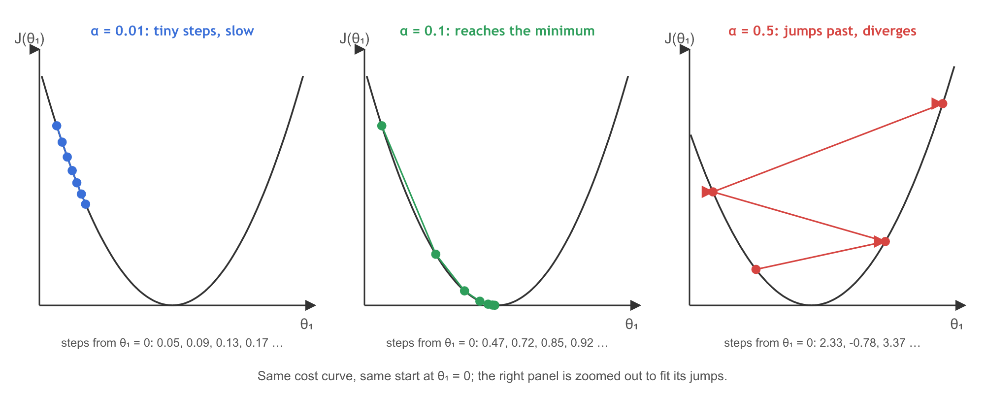
The learning rate α sets the speed of the walk to the global minimum:
- A small α takes small steps towards the minimum.
- A huge α makes the update jump from side to side, and θ₁ may never reach the global minimum.
- A very small α takes tiny steps, so training goes on for a very long time.
There is no single right value. The board writes α = 0.001 as an example of a small one; the runs below show what changing it does.
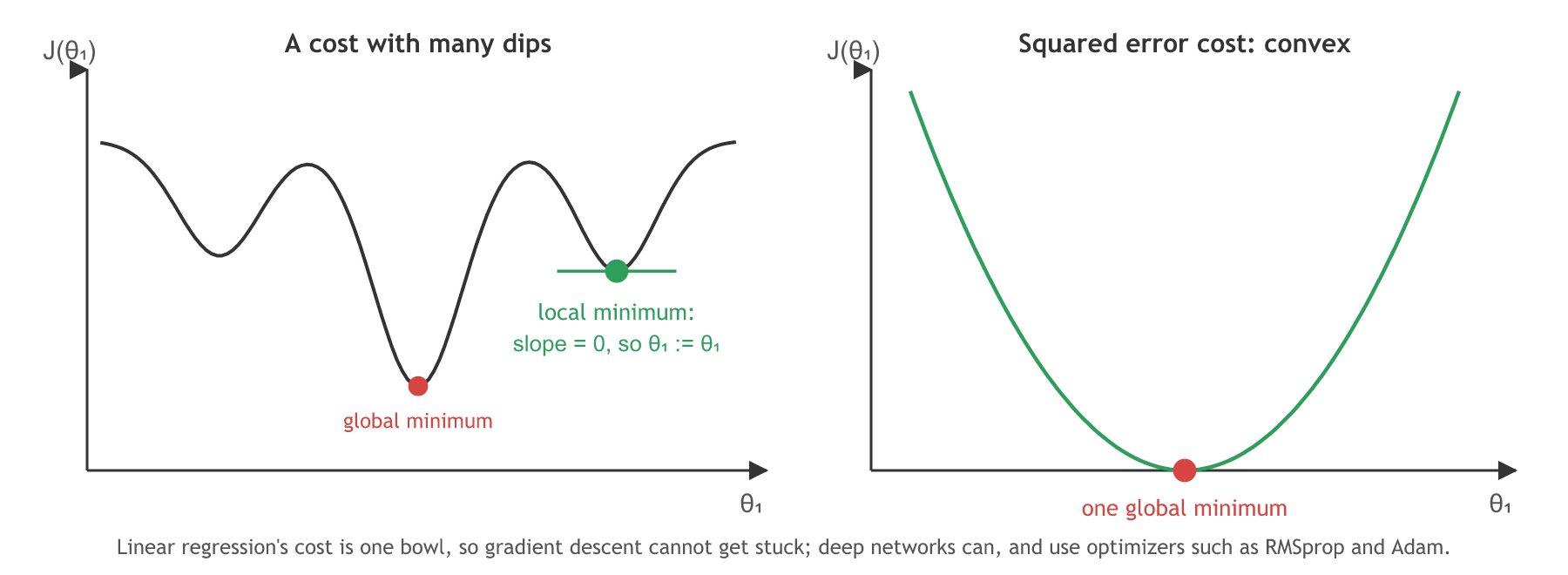
What if the cost had a local minimum, a dip that is not the lowest point? There the slope is zero, so the update becomes θ₁ := θ₁ and training gets stuck. The squared error cost of linear regression is convex, one bowl, so this does not happen. In deep learning, neural networks do have many local minima, and optimizers such as RMSprop and Adam handle them. The video flags this as an interview question: does linear regression have local minima? No. Convergence stops when J is very small and no longer falls.
Deriving the updates for θ0 and θ1
To run the rule, work out the derivative for j = 0 and j = 1. Apply it to the cost function: the derivative of (1/2m)·x² is (2/2m)·x, so the 2 cancels and 1/m is left. Then use hθ(x) = θ₀ + θ₁x: its derivative with respect to θ₀ is 1, and with respect to θ₁ it is x.
Midway through, the board writes the θ₁ derivative with the square still on the bracket, and the video removes it a moment later. The derivative has no square: the 2 from the square is the one that cancelled the 1/2.
With several features x₁, x₂, x₃, x₄ the cost becomes a bowl in more dimensions, and gradient descent is like coming down a mountain.
Running gradient descent in NumPy
Comparing three learning rates
First the board's three points (1,1), (2,2), (3,3) with hθ(x) = θ₁x, starting from θ₁ = 0, for six steps each:
import numpy as np

x = np.array([1.0, 2.0, 3.0])
y = np.array([1.0, 2.0, 3.0])

for alpha in [0.01, 0.1, 0.5]:
    theta1 = 0.0
    steps = []
    for _ in range(6):
        slope = np.mean((theta1 * x - y) * x)   # dJ/dθ1 for hθ(x) = θ1·x
        theta1 = theta1 - alpha * slope
        steps.append(f"{theta1:.2f}")
print(f"α = {alpha}:", ", ".join(steps))α = 0.01: 0.05, 0.09, 0.13, 0.17, 0.21, 0.25 α = 0.1: 0.47, 0.72, 0.85, 0.92, 0.96, 0.98 α = 0.5: 2.33, -0.78, 3.37, -2.16, 5.21, -4.62
One step for both parameters
Now both θ₀ and θ₁, on the age and weight table from Simple linear regression.
import numpy as np

x = np.array([24, 25, 21, 27], dtype=float)   # age
y = np.array([62, 63, 72, 62], dtype=float)   # weight

def gradients(theta0, theta1):
    error = theta0 + theta1 * x - y           # hθ(x) − y for every row
    return error.mean(), (error * x).mean()   # ∂J/∂θ0 and ∂J/∂θ1
Converging to the LinearRegression answer
from sklearn.linear_model import LinearRegression

theta0, theta1, alpha = 0.0, 0.0, 0.003
for step in range(1, 1_000_001):                 # repeat until convergence
    g0, g1 = gradients(theta0, theta1)
    theta0, theta1 = theta0 - alpha * g0, theta1 - alpha * g1   # update both together
    if abs(g0) < 1e-6 and abs(g1) < 1e-6:        # the slope is flat: converged
        break

print("steps:", step)
print("gradient descent: θ0 =", round(theta0, 2), " θ1 =", round(theta1, 3))
model = LinearRegression().fit(x.reshape(-1, 1), y)
print("LinearRegression: θ0 =", round(model.intercept_, 2), " θ1 =", round(model.coef_[0], 3))steps: 575671 gradient descent: θ0 = 105.81 θ1 = -1.693 LinearRegression: θ0 = 105.81 θ1 = -1.693
Reading the runs
- α = 0.01 crawls: after six steps θ₁ is only at 0.25. α = 0.1 is at 0.98 after six steps. α = 0.5 diverges: it overshoots from 0 to 2.33, then to −0.78, and each jump is bigger.
- 575,671 steps for the age table. The ages sit near 24, far from 0, so a change in θ₀ and a change in θ₁ pull in almost the same direction. The safe α is small (0.004 already diverges), and the walk along the long, flat valley of the cost takes many steps.
- The answer matches. Gradient descent lands on θ₀ = 105.81 and θ₁ = −1.693, the same line that
LinearRegressionfinds.
LinearRegression vs gradient descent
| LinearRegression | Gradient descent | |
|---|---|---|
| How θ is found | Solves least squares directly, in one go (Ordinary least squares) | Repeated small steps down the slope |
| Learning rate | None | Needs α; too big diverges, too small is slow |
| Work on the age table | One solve | 575,671 steps |
| Where it shines | Small and medium tables | Huge datasets and neural networks |
| In scikit-learn | LinearRegression | SGDRegressor (a stochastic version) |
Where you use gradient descent
- Training neural networks, where no direct solution exists, with optimizers such as Adam built on the same update.
- Very large tables, where
SGDRegressorupdates θ from small batches of rows. - Logistic regression, later in the course, which has no closed-form answer and is fitted by iterative solvers.
nan. Lower α by ten times before changing anything else.Related
- Previous: Cost function
- Next: Ordinary least squares
- Reference: SGDRegressor
- In the age run, change α to 0.004: θ0 and θ1 overflow and print
nan. - Change α to 0.001, the board's example value: the loop hits its 1,000,000-step cap first, still short of the answer (θ0 ≈ 105.77).
- In the three-point run, start from
theta1 = 2.5with α = 0.1: the slope is positive, so θ₁ falls: 1.80, 1.43, 1.23 and on towards 1.
Slow is fine. Stopping is the only problem.