Log loss
Log loss is the cost function of logistic regression: it charges −log(h) when the true class is 1 and −log(1 − h) when it is 0, which gives a convex curve that gradient descent can minimise.
Last updated: 05 Oct, 2026 · scikit-learn 1.9.1
Logistic regression needs a cost function to choose θ, as linear regression did in Cost function. The squared error does not work once the sigmoid is inside it, and this lesson shows why and what replaces it.
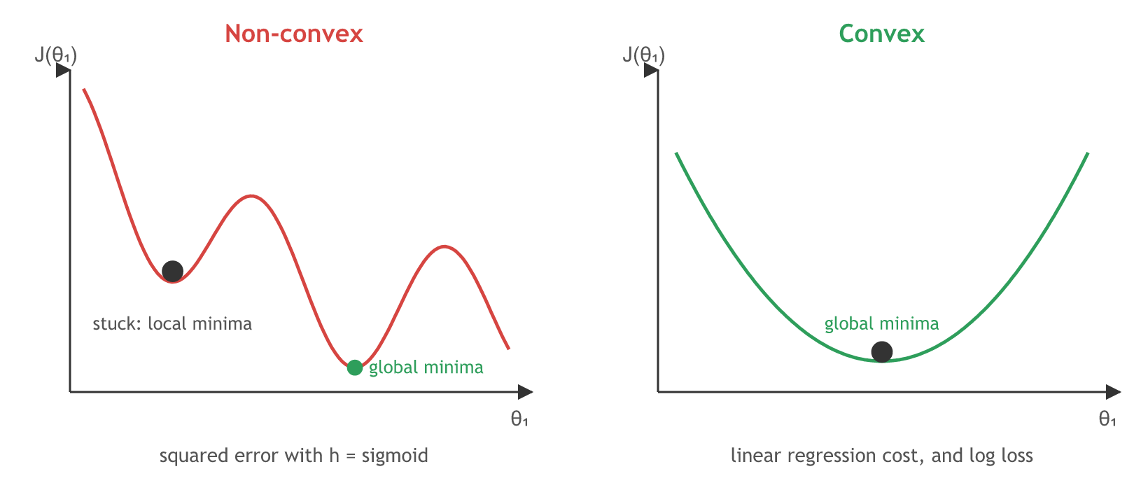
The board's arrow labels the sigmoid hypothesis itself "non convex function"; it is the squared-error cost built from it that is non-convex in θ₁.
Plugging the sigmoid into the squared error
The training set is {(x⁽¹⁾, y⁽¹⁾), (x⁽²⁾, y⁽²⁾), …, (x⁽ᵐ⁾, y⁽ᵐ⁾)} with every y either 0 or 1. To keep it simple the video sets θ₀ = 0, so z = θ₁x and θ₁ is the only parameter to change.
Linear regression's cost is J(θ₁) = (1/m) Σ ½ (hθ(x⁽ⁱ⁾) − y⁽ⁱ⁾)². Only hθ(x) changes for logistic regression: put the sigmoid in its place.
Seeing why the curve is non-convex
With linear regression's straight line, this cost is a parabola: a convex function, one bowl with one bottom, the global minima. With the sigmoid inside, the curve gets bumps. Where it has local minima, gradient descent can reach a dip that is not the lowest point; there the slope is 0, so θ₁ stops being updated and never reaches the global minima.
Writing the cost for y = 1 and y = 0
The cost that fixes it was proposed by researchers, and it uses the log. It is written in two cases, one for each value of y:
For y = 1 the curve of −log(h) is high when h is near 0 and falls to 0 at h = 1: "the cost will be zero if y = 1 and hθ(x) = 1". A confident right answer costs nothing; a confident wrong answer costs a lot. For y = 0 the curve is the mirror image, 0 at h = 0 and rising as h goes to 1. Both are convex, and so is their combination.
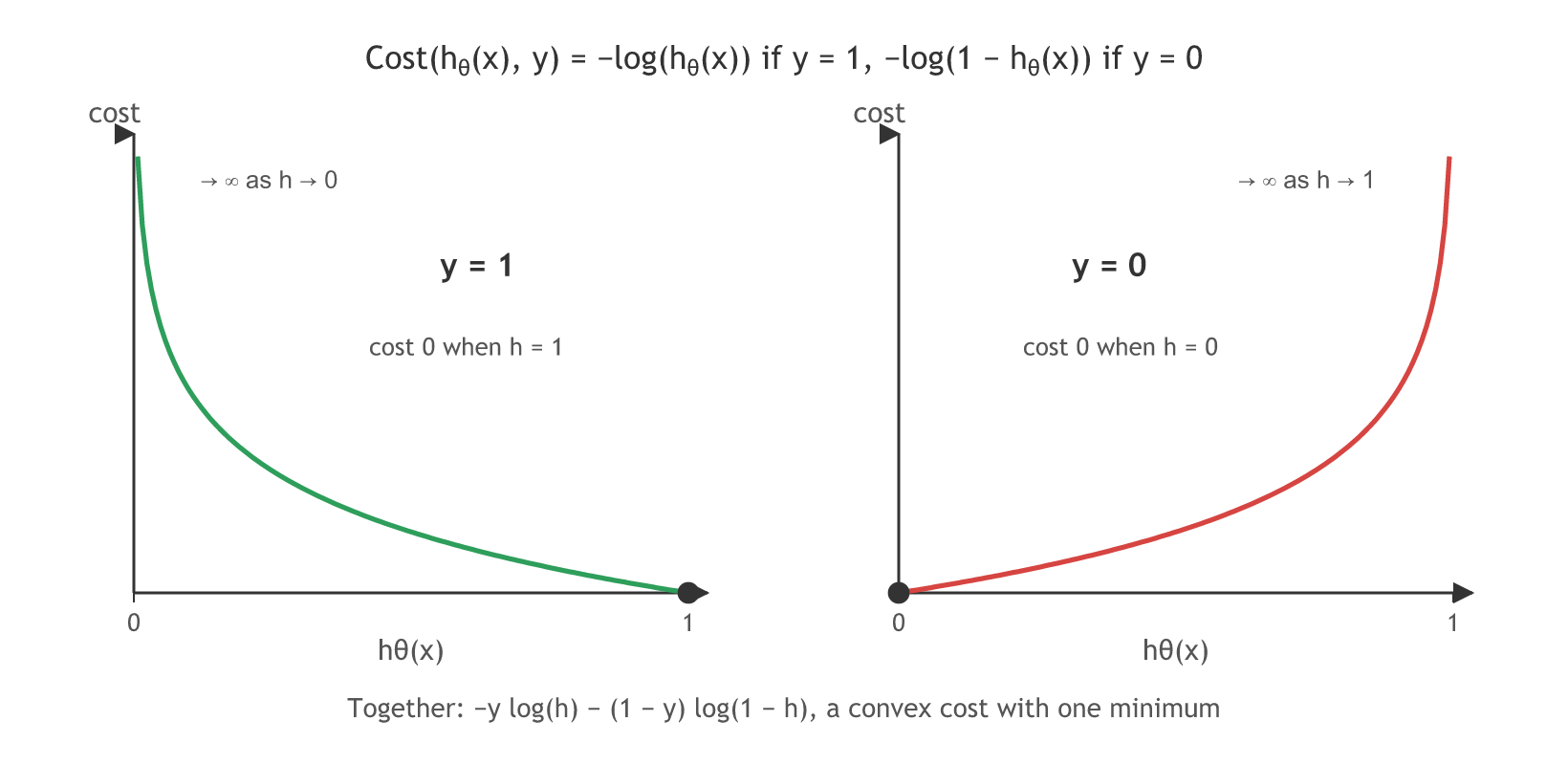
The board writes the average as −1/2m Σ; the standard log loss, and scikit-learn's log_loss, use 1/m. The ½ does not change which θ₁ is best, but it halves the number.
Combining the two cases into one formula
The two cases fit into one line. Put y = 1 and the second term vanishes, because 1 − y = 0, leaving −log(h). Put y = 0 and the first term vanishes, leaving −log(1 − h).
Averaged over the m training points, this is the log loss:
Training repeats the gradient descent update of Gradient descent until convergence. The video also answers a common question: yes, this is the log likelihood. Minimising log loss is the same as maximising the log likelihood of the labels.
Computing log loss in code
The log_loss function
sklearn.metrics.log_loss takes the true labels and the predicted probability of class 1 and returns the 1/m average.
from sklearn.metrics import log_loss

# y_true: the 0/1 labels, y_prob: the predicted P(class 1)
print(log_loss(y_true, y_prob))      # mean of -y log(p) - (1 - y) log(1 - p)
Log loss on the study hours, by hand and with scikit-learn
import numpy as np
from sklearn.linear_model import LogisticRegression
from sklearn.metrics import log_loss

hours = np.array([2, 3, 4, 5, 6, 7]).reshape(-1, 1)
result = np.array([0, 0, 0, 1, 1, 1])
h = LogisticRegression().fit(hours, result).predict_proba(hours)[:, 1]   # h for every student

cost = -result * np.log(h) - (1 - result) * np.log(1 - h)
print("h:   ", h.round(3))
print("cost:", cost.round(3))
print("1/m average  :", round(cost.mean(), 4))
print("log_loss     :", round(log_loss(result, h), 4))
print("board's 1/2m :", round(cost.sum() / (2 * len(result)), 4))h: [0.057 0.157 0.363 0.637 0.843 0.943] cost: [0.059 0.171 0.452 0.452 0.171 0.059] 1/m average : 0.2271 log_loss : 0.2271 board's 1/2m : 0.1136
Plotting both cost curves
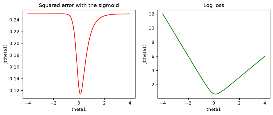
The second run plots both costs on the study hours with θ₀ = 0, as in the video, for θ₁ from −4 to 4. np.diff(curve, 2) is the change of the slope between neighbouring points; where it is negative, the curve bends downward, which a convex curve never does.
import numpy as np
import matplotlib.pyplot as plt

hours = np.array([2, 3, 4, 5, 6, 7])
result = np.array([0, 0, 0, 1, 1, 1])
theta1 = np.linspace(-4, 4, 801)                    # z = theta1 * x, theta0 = 0

def h(t):
    return 1 / (1 + np.exp(-t * hours))

squared = np.array([np.mean((h(t) - result) ** 2) / 2 for t in theta1])
logloss = np.array([-np.mean(result * np.log(h(t)) + (1 - result) * np.log(1 - h(t))) for t in theta1])

for name, curve in [("squared error", squared), ("log loss", logloss)]:
    bends_down = np.mean(np.diff(curve, 2) < -1e-12)
    print(f"{name:13}: lowest at theta1 = {theta1[curve.argmin()]:.2f}, bends downward on {bends_down:.0%} of the range")

fig, (left, right) = plt.subplots(1, 2, figsize=(10, 3.6))
left.plot(theta1, squared, color="red")
left.set_title("Squared error with the sigmoid")
right.plot(theta1, logloss, color="green")
right.set_title("Log loss")
for ax in (left, right):
    ax.set_xlabel("theta1")
    ax.set_ylabel("J(theta1)")
plt.show()squared error: lowest at theta1 = 0.12, bends downward on 63% of the range log loss : lowest at theta1 = 0.14, bends downward on 0% of the range
What the numbers and curves show
- log_loss matches the formula. The 1/m average by hand and
log_lossboth give 0.2271; the board's 1/2m gives half of it, 0.1136. - Confident and right costs little. The students at 2 and 7 hours have h = 0.057 (y = 0) and h = 0.943 (y = 1), a cost of 0.059 each. The students next to the boundary cost the most: 0.452 at 4 hours (h = 0.363, y = 0) and at 5 hours (h = 0.637, y = 1).
- The squared error is not a bowl. It bends downward on 63% of the range and goes flat at 0.25 on both sides. On a flat stretch the slope is near 0, so gradient descent started at θ₁ = −3 or 3 barely moves toward the dip. On these six points there is one dip, not the many local minima of the board's sketch, but the plateaus stall it the same way.
- Log loss is convex. It never bends downward (0%), so gradient descent from any start rolls into the same minimum.
Log loss vs squared error
| Squared error with the sigmoid | Log loss | |
|---|---|---|
| Formula per point | ½ (h − y)² | −y log h − (1 − y) log(1 − h) |
| Shape in θ | non-convex, flat plateaus | convex, one bowl |
| Confident wrong answer | costs at most ½ | cost grows without limit |
| Used for | linear regression | logistic regression, binary classifiers |
Where you use log loss
- Training logistic regression. scikit-learn's LogisticRegression minimises log loss, plus a penalty set by C.
- Comparing probability models. Two classifiers with the same accuracy can differ in log loss: the one with more honest probabilities scores lower.
- Neural networks. The same formula is called binary cross-entropy there.
log_loss(y, model.predict(X)) treats every 0 and 1 as a fully confident answer, so one mistake costs a huge amount; use model.predict_proba(X)[:, 1].Related
- Previous: Logistic regression
- Next: Confusion matrix
- Reference: scikit-learn: Log loss
- Change
resultin the first example to[0, 1, 0, 1, 1, 1], so the student at 3 hours passes and the one at 4 hours fails. No boundary splits them now, and the log loss rises from 0.2271 to 0.4296. - Print
-np.log(0.001)and-np.log(0.999): the cost of a confident wrong answer and of a confident right one. - In the second example, add an intercept: change
-t * hoursto-(t * hours - 4.5). The squared error still bends downward somewhere; log loss still never does.
Slow is fine. Stopping is the only problem.