Cost function
A cost function is a formula that measures how far a model's predictions are from the actual values, so training can pick the parameters that make it smallest.
Last updated: 05 Oct, 2026 · scikit-learn 1.9.1
The line from Simple linear regression has two numbers to choose, θ₀ and θ₁. The cost function turns each choice into one score, which gives "best fit" a precise meaning: the line with the lowest cost.
Measuring the distance to the line
The aim is a line where the distance between each data point and its predicted point is small, and the sum of all those distances is minimal. One could draw many lines and keep the one with the smallest total, but how many lines would that take? Instead, start at one point and move towards the best fit line. The cost function is what tells you which way is better.
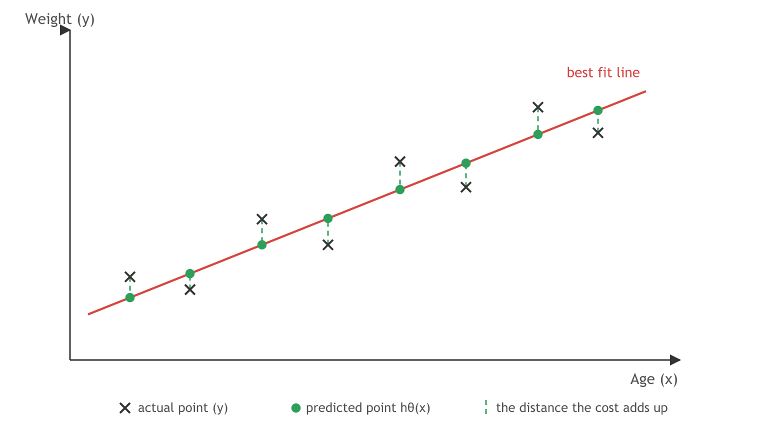
The distance is hθ(x) − y: the predicted point minus the real point. It is squared, because some differences are negative. It is summed over every point, i = 1 to m, where m is the number of data points. Then it is divided by 2m:
- 1/m turns the sum into an average.
- 1/2 is there for the derivation: the derivative of x² is 2x, and the 2 cancels the 1/2. Training takes this derivative when it updates θ₀ and θ₁.
- The square keeps every distance positive.
The notes write this J and label it the mean squared error. Strictly, the mean squared error has no 1/2: it is 2 × J, as MSE, MAE and RMSE shows. The 1/2 changes the size of J, never which θ₀ and θ₁ make it smallest.
Training means changing θ₀ and θ₁ until J is as small as it can be:
Simplifying to a line through the origin
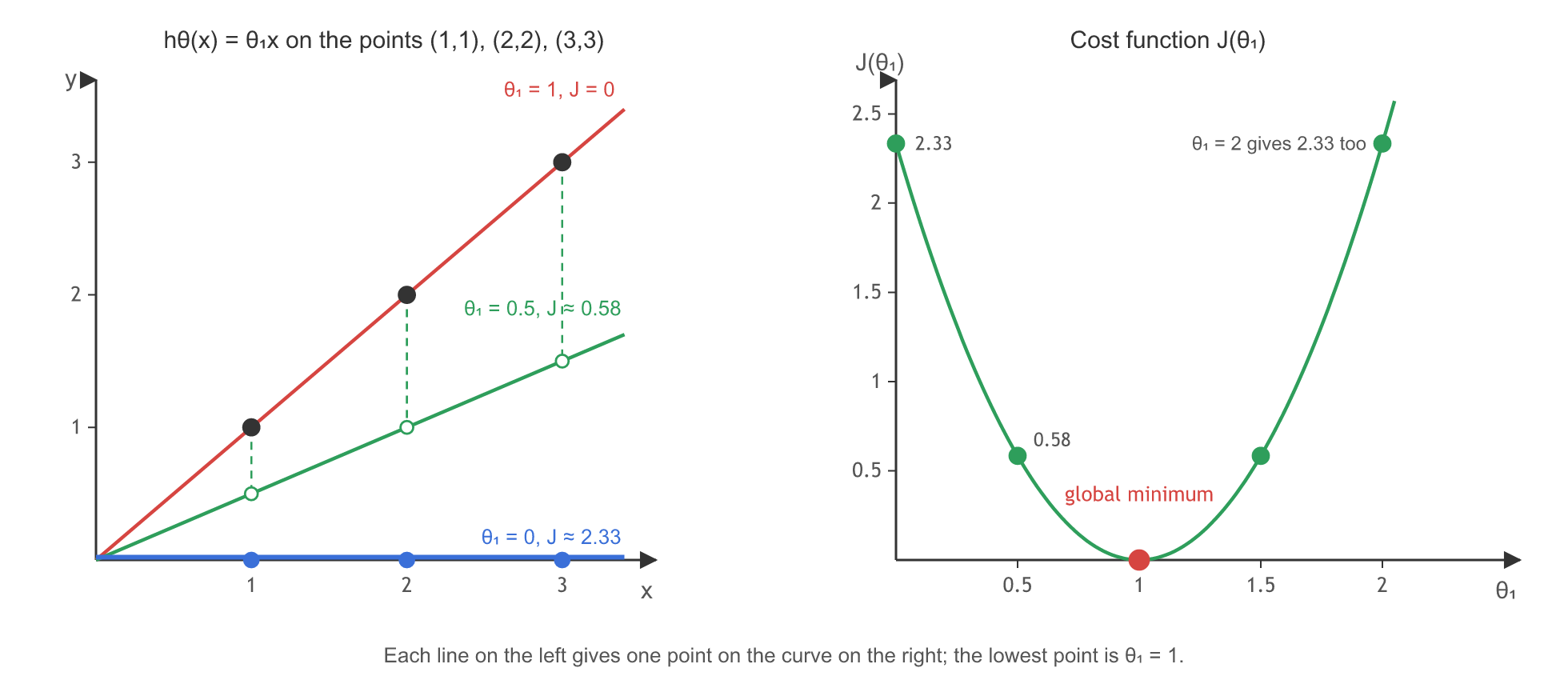
To see the cost on paper, set θ₀ = 0. The line then passes through the origin, and the hypothesis has one parameter: hθ(x) = θ₁x. Take three data points, (1,1), (2,2) and (3,3).
With θ₁ = 1 (slope 1), the line passes through all three points. Each prediction equals the real value, so every distance is zero:
That gives the first point of the cost graph: θ₁ = 1 on the horizontal axis, J(θ₁) = 0 on the vertical axis.
Computing J for θ1 = 0.5 and θ1 = 0
With θ₁ = 0.5 the predictions are 0.5 × 1 = 0.5, 0.5 × 2 = 1 and 0.5 × 3 = 1.5, the green line with a smaller slope:
With θ₁ = 0 every prediction is 0, so the line lies on the x axis:
Plot each pair (θ₁, J) and join the points: the result is a U-shaped curve. The board labels this curve "gradient descent"; the curve is the cost function J(θ₁), and gradient descent is the method that walks down it, in the next lesson. The lowest point, θ₁ = 1 with J = 0, is the global minimum: there the distance between the predicted and the real points is smallest, and the line is the best fit line.
Computing the cost in NumPy
The cost as a Python function
import numpy as np

x = np.array([1, 2, 3])
y = np.array([1, 2, 3])

def cost(theta1):
    predictions = theta1 * x                 # hθ(x) = θ1·x, the line through the origin
    return np.sum((predictions - y) ** 2) / (2 * len(x))
Reproducing the board's three costs
for theta1 in [1, 0.5, 0]:
    print(f"J({theta1}) = {cost(theta1):.3f}")
print("θ1 = 2 gives", round(cost(2), 3), "and θ1 = 1.5 gives", round(cost(1.5), 3))J(1) = 0.000 J(0.5) = 0.583 J(0) = 2.333 θ1 = 2 gives 2.333 and θ1 = 1.5 gives 0.583
Plotting the cost curve
import matplotlib.pyplot as plt

thetas = np.linspace(-0.5, 2.5, 61)
costs = [cost(t) for t in thetas]
plt.plot(thetas, costs, color="green")
plt.scatter([0, 0.5, 1], [cost(0), cost(0.5), cost(1)], color="red", zorder=3)
plt.title("Cost function J(θ1)")
plt.xlabel("θ1")
plt.ylabel("J(θ1)")
plt.show()
print("lowest cost on the grid at θ1 =", round(thetas[np.argmin(costs)], 2))lowest cost on the grid at θ1 = 1.0
What the costs and the curve show
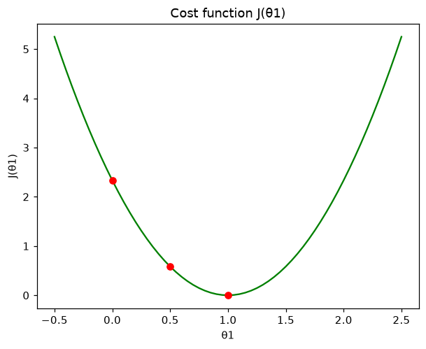
- 0.000, 0.583, 2.333 are the board's 0, 0.58 and 2.3, unrounded: 3.5 / 6 and 14 / 6.
- θ₁ = 2 and θ₁ = 1.5 mirror θ₁ = 0 and θ₁ = 0.5. The curve is symmetric around θ₁ = 1, so a line that is too steep costs as much as one that is equally too flat.
- The grid's lowest point is θ₁ = 1, the global minimum, and the curve has no other dip.
Squared error vs absolute error
| Squared error (this lesson) | Absolute error | |
|---|---|---|
| Per point | (hθ(x) − y)² | |hθ(x) − y| |
| Negative differences | Made positive by the square | Made positive by the absolute value |
| Large errors | Weigh much more (an error of 3 costs 9) | Weigh in proportion (an error of 3 costs 3) |
| Derivative | Smooth everywhere, so gradient descent is easy | Undefined at zero error |
| In scikit-learn | LinearRegression, mean_squared_error | mean_absolute_error |
Where you use the cost function
- Training: every regression model in this part minimises a cost like J.
- Comparing two candidate lines on the same data: the lower cost wins.
- Reading error metrics: scikit-learn's mean squared error is the same sum without the 1/2, so it equals 2 × J; MSE, MAE and RMSE compares it with the absolute error.
mean_squared_error is 1.167.Related
- Previous: Simple linear regression
- Next: Gradient descent
- Add a fourth point (4, 4) to
xandy: J(0.5) becomes (0.25 + 1 + 2.25 + 4) / 8 = 0.9375. - Change the last point to (3, 4) and replot: the lowest cost moves to about θ₁ = 1.2.
- Import
mean_squared_errorfromsklearn.metricsand check thatmean_squared_error(y, 0.5 * x)equals2 * cost(0.5).
You understood something today that you didn't yesterday.