MSE, MAE and RMSE
MSE, MAE and RMSE are regression performance metrics that average the gaps between actual and predicted values: the mean squared error squares each gap, the mean absolute error takes its size, and the root mean squared error is the square root of the MSE.
Last updated: 05 Oct, 2026 · scikit-learn 1.9.1
R squared and adjusted R squared says what share of the variation a model explains. These three say how far off the predictions are, in the output's own terms, such as lakhs of salary or centimetres of height. The notes list five metrics for a regression model: MSE, MAE, RMSE, R² and adjusted R².
Squaring the errors with MSE
This is the cost function from Cost function without the 1/2. It is a quadratic equation in the parameters, and the notes list what follows from that:
- Advantage: differentiable. Its graph is a smooth convex curve, so gradient descent can take the slope anywhere.
- Advantage: one minimum. The notes write "one local and one global minima": for a convex curve they are the same single point, so there is no dip to get stuck in.
- Advantage: it converges faster, because the slope shrinks as the error shrinks.
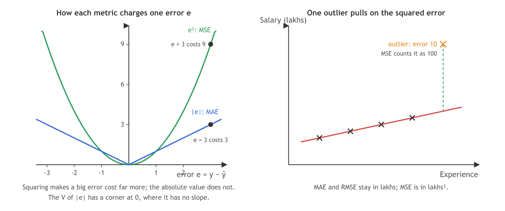
- Disadvantage: outliers. Squaring penalises a big error heavily. One salary far from the line adds its error squared and drags the fitted line towards it.
- Disadvantage: not in the same unit. With salary in lakhs, MSE is in lakhs squared, so an MSE of 2.5 does not read as 2.5 lakhs.
Taking the size of the errors with MAE
- Advantage: less pulled by outliers. Each error counts in proportion: an error of 10 adds 10, not 100.
- Advantage: the same unit as the output: an MAE of 0.3 means predictions are off by 0.3 lakhs on average.
- Disadvantage: harder to optimise. |e| has a sharp corner at 0, where it has no derivative, so optimisers use a subgradient there. Convergence usually takes more time.
Returning to the same unit with RMSE
- Advantages: the same unit as the output, and differentiable.
- Disadvantage: still sensitive to outliers, because the errors are squared before the root.
Working the three metrics by hand
Five salaries in lakhs and a model's predictions:
| Actual y | Predicted ŷ | Error y − ŷ | Squared | Absolute |
|---|---|---|---|---|
| 4 | 4.5 | −0.5 | 0.25 | 0.5 |
| 5 | 5 | 0 | 0 | 0 |
| 6 | 5.5 | 0.5 | 0.25 | 0.5 |
| 7 | 7.5 | −0.5 | 0.25 | 0.5 |
| 8 | 8 | 0 | 0 | 0 |
| Sum | 0.75 | 1.5 |
MSE = 0.75 / 5 = 0.15 lakhs², MAE = 1.5 / 5 = 0.3 lakhs, RMSE = √0.15 ≈ 0.387 lakhs. Now make the last salary an outlier, 18 instead of 8, with the same prediction of 8. Its error is 10: the squared sum becomes 100.75 and the absolute sum 11.5, so MSE = 20.15, MAE = 2.3 and RMSE ≈ 4.489.
Computing the metrics in scikit-learn
The three metric functions
import numpy as np
from sklearn.metrics import mean_squared_error, mean_absolute_error, root_mean_squared_error

actual = np.array([4, 5, 6, 7, 8])            # salary in lakhs
predicted = np.array([4.5, 5, 5.5, 7.5, 8])   # a model's predictions

def report(y_true, y_pred):
    print("MSE :", round(mean_squared_error(y_true, y_pred), 3))
    print("MAE :", round(mean_absolute_error(y_true, y_pred), 3))
    print("RMSE:", round(root_mean_squared_error(y_true, y_pred), 3))
Adding one outlier
report(actual, predicted)
print("--- the last salary is an outlier: 18 instead of 8")
with_outlier = actual.copy()
with_outlier[-1] = 18
report(with_outlier, predicted)MSE : 0.15 MAE : 0.3 RMSE: 0.387 --- the last salary is an outlier: 18 instead of 8 MSE : 20.15 MAE : 2.3 RMSE: 4.489
Scoring the height model from the practical notebook
The practical notebook scores its height and weight line from Simple linear regression with all five metrics. It computes RMSE as np.sqrt(mse), which gives the same number as root_mean_squared_error:
import numpy as np
from sklearn.metrics import mean_squared_error, mean_absolute_error, r2_score

y_pred = regression.predict(X_test)
mse = mean_squared_error(y_test, y_pred)
mae = mean_absolute_error(y_test, y_pred)
rmse = np.sqrt(mse)
print("MSE:", round(mse, 2), " MAE:", round(mae, 3), " RMSE:", round(rmse, 3))

score = r2_score(y_test, y_pred)
n, p = X_test.shape   # 6 test rows, 1 feature
print("R²:", round(score, 4), " adjusted R²:", round(1 - (1 - score) * (n - 1) / (n - p - 1), 4))MSE: 114.84 MAE: 9.665 RMSE: 10.716 R²: 0.7361 adjusted R²: 0.6701
What the metrics printed
- One outlier multiplies MSE by about 134 (0.15 to 20.15) but MAE only by about 8 (0.3 to 2.3). That is the squaring at work, and the reason MAE is preferred when a few wild rows should not dominate.
- RMSE sits between them (0.387 to 4.489) and is in lakhs like MAE. RMSE is never smaller than MAE; the two are equal only when every error has the same size.
- The height model is off by about 10 cm: MAE 9.665 cm and RMSE 10.716 cm, while MSE reads 114.84 cm². R² is 0.7361 and adjusted R² 0.6701, the notebook's own five numbers.
MSE vs MAE vs RMSE
| MSE | MAE | RMSE | |
|---|---|---|---|
| Formula | mean of (y − ŷ)² | mean of |y − ŷ| | √MSE |
| Unit | Output unit squared | Output unit | Output unit |
| Outliers | Weigh heavily | Weigh in proportion | Weigh heavily |
| Differentiable at 0 error | Yes | No, a subgradient is used | Yes |
| In scikit-learn | mean_squared_error | mean_absolute_error | root_mean_squared_error |
| As a scorer | neg_mean_squared_error | neg_mean_absolute_error | neg_root_mean_squared_error |
Where you use MSE, MAE and RMSE
- Training: MSE is the loss most regression models minimise, because it is smooth.
- Reporting to people: MAE or RMSE, in the output's own unit: "the price is off by 0.3 lakhs on average".
- Comparing models: pass a scorer name such as
neg_root_mean_squared_errortocross_val_score, as Cross-validation does with the MSE scorer.
Related
- Previous: R squared and adjusted R squared
- Next: Multiple linear regression
- Reference: Regression metrics in the scikit-learn user guide
- Make the outlier 28 instead of 18: MSE grows to 80.15 while MAE grows only to 4.3.
- Import
median_absolute_errorand report it too: with one outlier among five rows it stays at 0.5. - Set every prediction 1 lakh too high (
predicted = actual + 1): MAE and RMSE both print 1.0, the case where they are equal.
Little by little, you're building something great.