K-means clustering
K-means clustering is an unsupervised learning algorithm that splits data into K groups, each one built around a centre point called a centroid.
Last updated: 05 Oct, 2026 · scikit-learn 1.9.1
Support vector machines (SVM) learned from a label on every row. Unsupervised learning has no output column at all, only the features, and clustering finds which rows are similar. K-means is the first clustering algorithm, and the one used most.
Grouping data with no output column
In unsupervised machine learning there is no specific output. The board has two features, f1 and f2, and the points fall into two groups of similar data, cluster 1 and cluster 2. Finding those groups is clustering, and the video names the techniques: K-means first, then hierarchical clustering.
The video gives a use straight away: a custom ensemble clusters the data into two or three groups first, then trains a separate supervised model on each group.
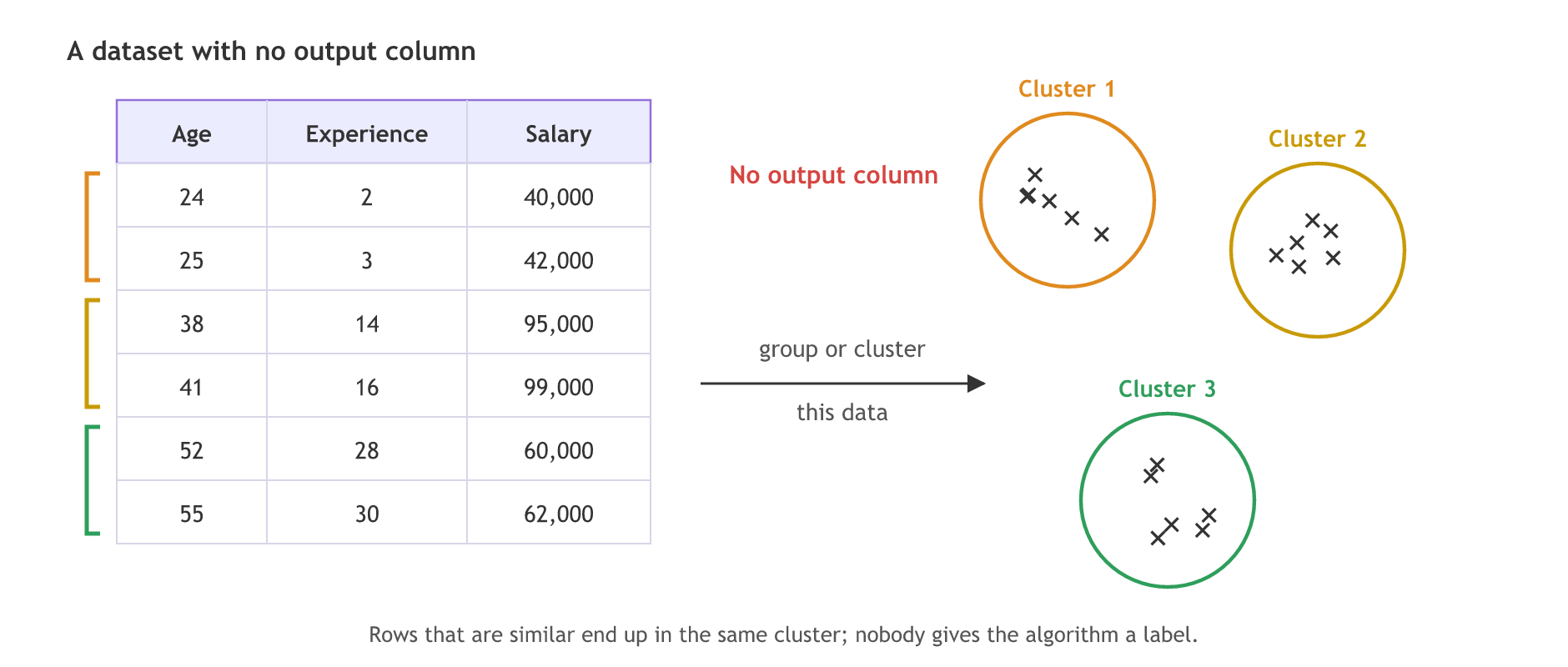
The board notes for this part draw the same idea as a table of age, experience and salary with no output column, where similar rows form clusters. Customer segmentation is the usual case: a company launching a new product groups its customers by salary and spending score, then gives each group its own offer, such as a 15% discount for one group and 20% for another. Supervised and unsupervised learning has a salary and age example of the same kind.
The notes list the tools this part teaches:
- K-means, this lesson: K centroids, each point joins the nearest one.
- Hierarchical clustering: merges the nearest points into a tree.
- DBSCAN: grows clusters out of dense regions and leaves outliers out.
- Silhouette score: validates the clusters any of the three makes.
Choosing K and placing the centroids
K is the number of clusters. Every cluster has one centroid, so K is also the number of centroids; the board shortens this to "K = centroids". On the board two groups are easy to see, so K = 2. Real data has many features and cannot be plotted, so nobody can count the groups by eye. That is why K-means starts by trying different K values.
- Choose a value of K (the elbow method below is how).
- Place K centroids at random positions among the points.
Assigning points and moving the centroids
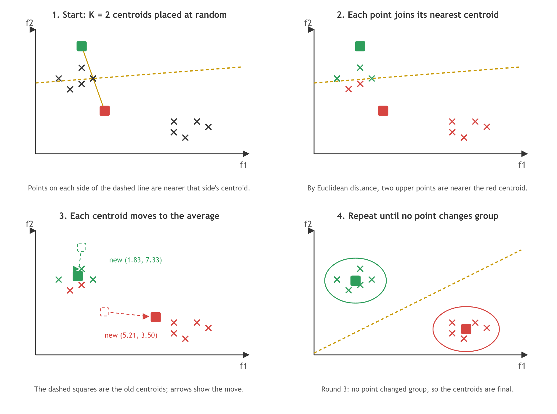
Next, every point is measured against every centroid with Euclidean distance and joins the nearest one. The board uses a shortcut for two centroids: join them with a line, then draw a second line across its middle at a right angle. Every point on the green side is nearer the green centroid, every point on the red side nearer the red one.
Then each centroid moves to the average of the points that joined it. With the centroids in new places, the distances are measured again and some points may switch sides. The loop stops when no point changes group, because then no centroid moves either.
The board notes give two ways to measure the distance. Euclidean distance is the straight line, like a flight path between two cities. Manhattan distance walks along the streets of a grid, block by block. scikit-learn's KMeans always uses Euclidean distance: the centroid update takes the average, and the average is the point with the smallest sum of squared Euclidean distances to its group. K nearest neighbours (KNN) lets you choose between the two.
The diagram runs these steps on ten points. The random start puts the green centroid at (2, 10) and the red one at (3, 4). The loop below repeats the steps with NumPy and prints every round.
import numpy as np

# Ten points in two groups, like the board: upper left and lower right
X = np.array([[1, 7], [2, 8], [1.5, 6], [2.5, 7], [2, 6.5],
              [6, 2], [7, 3], [6.5, 1.5], [7.5, 2.5], [6, 3]])
centroids = np.array([[2.0, 10.0], [3.0, 4.0]])   # K = 2 random starts: green, red

for round_no in range(1, 10):
    # Euclidean distance from every point to every centroid
    dist = np.sqrt(((X[:, None, :] - centroids[None, :, :]) ** 2).sum(axis=2))
    groups = dist.argmin(axis=1)                    # 0 = green, 1 = red
    # Move each centroid to the average of its points
    new = np.array([X[groups == k].mean(axis=0) for k in range(2)])
    print(f"round {round_no}: groups {groups}, centroids {new.round(2).tolist()}")
    if np.allclose(new, centroids):                 # nothing moved: stop
        break
centroids = newround 1: groups [0 0 1 0 1 1 1 1 1 1], centroids [[1.83, 7.33], [5.21, 3.5]] round 2: groups [0 0 0 0 0 1 1 1 1 1], centroids [[1.8, 6.9], [6.6, 2.4]] round 3: groups [0 0 0 0 0 1 1 1 1 1], centroids [[1.8, 6.9], [6.6, 2.4]]
- Round 1 puts two of the upper points, (1.5, 6) and (2, 6.5), in the red group, so the red average lands between the two groups at (5.21, 3.5).
- Round 2 measures again from the moved centroids: both points switch to green, and the centroids move to (1.8, 6.9) and (6.6, 2.4).
- Round 3 changes no point, so the centroids stay where they are and the loop stops.
Choosing K with the elbow method
The elbow method tries K = 1 to 10 and records the within cluster sum of squares (WCSS) for each K: the squared distance from every point to its own centroid, added up. With K = 1 one centroid serves every point, so the distances are long and WCSS is large. With K = 2 each point has a nearer centroid, so WCSS drops.
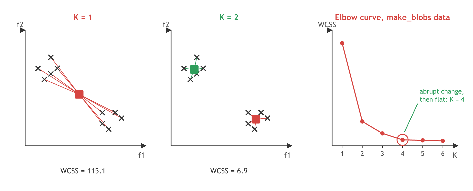
Plotted against K, WCSS falls fast and then flattens. Where the abrupt fall turns into a nearly straight line the curve looks like an elbow, and that K is the one to pick; the board circles K = 4. The elbow only picks K. Checking that the clusters are good is the job of the Silhouette score.
Avoiding a bad start with k-means++
The video then names a weakness: the starting centroids are random. A bad start can split one real group across two centroids, and the loop cannot repair it, because it stops as soon as no point changes group, even when a better grouping exists. The board writes K = 2 but draws three starting centroids: the picture shows a run where one real group is split across two centroids. The board notes draw the same trap with K = 3 on two real groups: wherever the random centroids land, one real group ends up cut in two.
The fix is k-means++, which places the starting centroids far apart. The first one is a random data point; each next one is drawn with a higher chance the farther a point is from the centroids already chosen.
Fitting K-means on the make_blobs data
The practical makes its own data with make_blobs: 500 points, two features and four centres. The notebook's comment says the setting has one distinct cluster and three clusters placed close together, which is what makes choosing K interesting.
The video ran on an older scikit-learn. Since version 1.4, KMeans runs the algorithm once by default (n_init="auto" with the k-means++ start) instead of ten times. The elbow curve keeps the video's shape; where the change shows in the numbers is covered in Silhouette score.
Generating the make_blobs data
from sklearn.datasets import make_blobs

# 500 points, 2 features, 4 centres inside the box -10 to 10
X, y = make_blobs(n_samples=500, n_features=2, centers=4, cluster_std=1,
                  center_box=(-10.0, 10.0), shuffle=True, random_state=1)
print(X.shape, y.shape)   # y is the true blob, which clustering never sees
Reading inertia_ for each K
inertia_ is scikit-learn's name for WCSS: after fit it holds the sum of squared distances from each point to its nearest centroid.
from sklearn.cluster import KMeans

wcss = []
for i in range(1, 11):
    kmeans = KMeans(n_clusters=i, init="k-means++", random_state=0)
    kmeans.fit(X)
    wcss.append(kmeans.inertia_)   # WCSS for this K
The elbow curve for K = 1 to 10
from sklearn.datasets import make_blobs
from sklearn.cluster import KMeans
import matplotlib.pyplot as plt

X, y = make_blobs(n_samples=500, n_features=2, centers=4, cluster_std=1,
                  center_box=(-10.0, 10.0), shuffle=True, random_state=1)

wcss = []
for i in range(1, 11):
    kmeans = KMeans(n_clusters=i, init="k-means++", random_state=0)
    kmeans.fit(X)
    wcss.append(kmeans.inertia_)

print([round(w, 1) for w in wcss])
plt.plot(range(1, 11), wcss)
plt.title("The Elbow Method")
plt.xlabel("Number of Clusters")
plt.ylabel("WCSS")
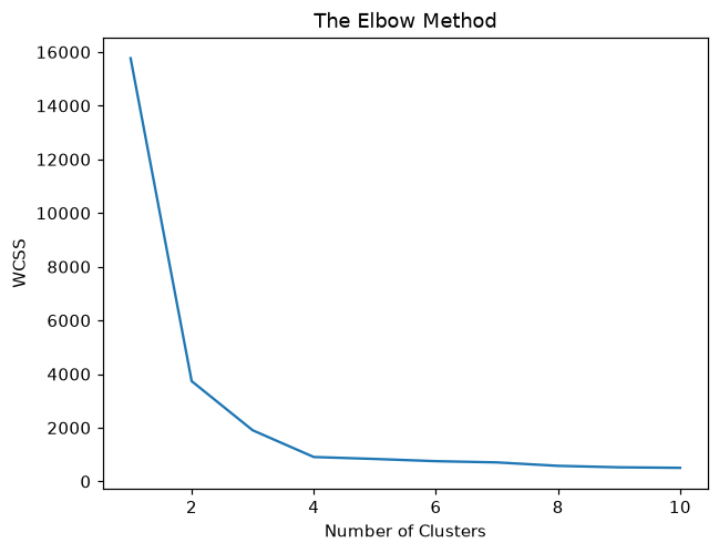
plt.show()[15767.6, 3735.4, 1903.7, 908.4, 835.6, 752.7, 706.9, 578.8, 524.9, 504.4]
Reading the elbow curve
- K = 1 to 2 drops WCSS from 15767.6 to 3735.4: the distinct cluster gets its own centroid.
- K = 3 and 4 keep falling, to 1903.7 and 908.4, as the three close blobs get one centroid each.
- After K = 4 the curve is nearly flat (835.6 at K = 5): extra centroids only cut real groups in pieces. The elbow is K = 4, the same choice as the video.
Fitting the final model with K = 4
The video then fits the chosen model with the same call the silhouette code uses, KMeans(n_clusters=4, random_state=10), and reads one label per point from fit_predict.
from sklearn.cluster import KMeans
import numpy as np

clusterer = KMeans(n_clusters=4, random_state=10)
cluster_labels = clusterer.fit_predict(X)
print(cluster_labels[:20])
print("points per cluster:", np.bincount(cluster_labels))
print("centroids:")
print(clusterer.cluster_centers_.round(2))
print("WCSS:", round(clusterer.inertia_, 1))[3 3 0 1 2 1 2 2 2 2 3 3 2 1 2 3 2 3 1 2] points per cluster: [128 125 123 124] centroids: [[-10.01 -3.85] [ -1.54 4.44] [ -6.08 -3.17] [ -7.09 -8.11]] WCSS: 908.4
Random starts against k-means++
The video promises to show k-means++ in the practical; this run does it with numbers. It fits the same data ten times from purely random starts and ten times from k-means++ starts, one run each (n_init=1), and plots the worst random run beside a k-means++ run.
from sklearn.cluster import KMeans
import matplotlib.pyplot as plt

# Ten single runs (n_init=1) from each kind of start
random_runs = [KMeans(n_clusters=4, init="random", n_init=1, random_state=s).fit(X)
               for s in range(10)]
plus_runs = [KMeans(n_clusters=4, init="k-means++", n_init=1, random_state=s).fit(X)
             for s in range(10)]
print("random   :", [round(m.inertia_, 1) for m in random_runs])
print("k-means++:", [round(m.inertia_, 1) for m in plus_runs])

bad = max(random_runs, key=lambda m: m.inertia_)    # the worst random start
fig, (ax1, ax2) = plt.subplots(1, 2, figsize=(11, 4.5))
for ax, m, name in [(ax1, bad, "Random start"), (ax2, plus_runs[0], "k-means++ start")]:
    ax.scatter(X[:, 0], X[:, 1], c=m.labels_, s=12, cmap="viridis")
    ax.scatter(m.cluster_centers_[:, 0], m.cluster_centers_[:, 1], c="red", marker="x", s=150)
    ax.set_title(f"{name}: WCSS {m.inertia_:.1f}")
    ax.set_xlabel("Feature 1")
    ax.set_ylabel("Feature 2")
plt.show()random : [908.4, 1806.2, 908.4, 3609.8, 1819.8, 908.4, 908.4, 1819.6, 908.5, 908.4] k-means++: [908.4, 908.4, 908.4, 908.4, 908.4, 908.4, 908.4, 908.4, 908.4, 908.4]
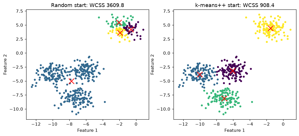
What the random starts show
- Six of the ten random starts reach WCSS 908.4 (or 908.5), the same answer as the elbow run.
- Four random starts get stuck at 1806.2, 1819.8, 1819.6 or 3609.8: a real blob is split across centroids while other blobs share one, the trap the board draws. In the worst run, three centroids sit in the distinct blob and one centroid covers the three close blobs.
- All ten k-means++ starts reach 908.4. That is why k-means++ is the default init, and why the default runs more than one start when the init is random.
Scaling the features and labelling new points
The K-means notebook in the course materials takes one more step. It makes 1,000 points around 3 centres, splits them with train_test_split, scales the features with StandardScaler, and runs the elbow method on the scaled training rows. The fitted model then labels the test rows with predict(): each new point joins its nearest centroid, and the centroids do not move.
Scaling on the training rows only
The scaler learns the mean and standard deviation from the training rows, then applies the same numbers to the test rows, so the test rows stay unseen.
from sklearn.preprocessing import StandardScaler

scaler = StandardScaler()
X_train_scaled = scaler.fit_transform(X_train)   # learn mean and std, then scale
X_test_scaled = scaler.transform(X_test)         # reuse the training numbers
Labelling the test rows with predict
kmeans = KMeans(n_clusters=3, init="k-means++", random_state=42)
kmeans.fit_predict(X_train_scaled)       # cluster the training rows
y_pred = kmeans.predict(X_test_scaled)   # nearest centroid for each new point
Clustering 1,000 scaled points into 3 groups
The notebook sets no random_state, so its numbers change on every run; the code here fixes random_state=42. The notebook also finds the elbow automatically with KneeLocator from the separate kneed package, which reports K = 3. Here the WCSS list is read by eye.
import numpy as np
import matplotlib.pyplot as plt
from sklearn.datasets import make_blobs
from sklearn.model_selection import train_test_split
from sklearn.preprocessing import StandardScaler
from sklearn.cluster import KMeans

X, y = make_blobs(n_samples=1000, centers=3, n_features=2, random_state=42)
X_train, X_test, y_train, y_test = train_test_split(X, y, test_size=0.33, random_state=42)

scaler = StandardScaler()
X_train_scaled = scaler.fit_transform(X_train)
X_test_scaled = scaler.transform(X_test)

wcss = []
for k in range(1, 11):
    kmeans = KMeans(n_clusters=k, init="k-means++", random_state=42)
    kmeans.fit(X_train_scaled)
    wcss.append(kmeans.inertia_)
print("WCSS:", [round(w, 1) for w in wcss])

kmeans = KMeans(n_clusters=3, init="k-means++", random_state=42)
train_labels = kmeans.fit_predict(X_train_scaled)
y_pred = kmeans.predict(X_test_scaled)
print("training rows per cluster:", np.bincount(train_labels))
print("test rows per cluster:    ", np.bincount(y_pred))

plt.scatter(X_test[:, 0], X_test[:, 1], c=y_pred)
plt.title("Test points labelled by predict()")
plt.xlabel("Feature 1")
plt.ylabel("Feature 2")
plt.show()WCSS: [1340.0, 424.8, 43.5, 36.8, 30.9, 28.5, 23.4, 21.5, 19.5, 17.4] training rows per cluster: [219 219 232] test rows per cluster: [114 114 102]
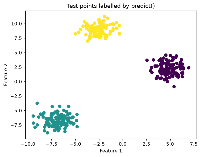
What the scaled run shows
- WCSS falls from 1340.0 to 424.8 and then to 43.5 at K = 3; after that it barely moves. The elbow is K = 3, the number of centres make_blobs used.
- WCSS at K = 1 is 1340.0, the same as in the notebook: after scaling, each feature of the 670 training rows has variance 1, so one centroid at the mean gives 670 × 2 = 1340.
- predict() labels the 330 test rows into three groups of similar size, and the plot shows each blob in one colour.
Random initialisation vs k-means++
| Random initialisation | k-means++ | |
|---|---|---|
| Starting centroids | K data points picked at random | spread out: a far point is more likely to be picked |
| Ten single runs on make_blobs | 4 of 10 end at a worse WCSS | 10 of 10 end at WCSS 908.4 |
| scikit-learn setting | init="random" | init="k-means++", the default |
Where you use K-means clustering
- Customer segments: group shoppers by spend and visits, then plan offers per group.
- The custom ensemble from the video: cluster first, then train one supervised model per group.
- Image colours: cluster the pixel colours into K centroids and repaint every pixel with its centroid's colour.
Related
- Previous: SVM kernels
- Next: Hierarchical clustering
- Reference: scikit-learn user guide: K-means
- In the NumPy loop, start the centroids at [[1.0, 1.0], [8.0, 8.0]], a start far from both groups, and count the rounds before it stops.
- In the random-start example, change n_init=1 to n_init=10 for the random starts and check that every run now ends near 908.4.
- In the elbow example, change centers=4 to centers=3 in make_blobs and see where the elbow moves.
Every expert started right here.