K nearest neighbours (KNN)
K nearest neighbours (KNN) is a supervised learning algorithm that predicts a new point from the K training points closest to it: a majority vote for classification, an average for regression.
Last updated: 04 Oct, 2026 · scikit-learn 1.9.1
Naive Bayes worked example predicted from counts. KNN needs no formula to fit at all: it keeps the training points and, for each new point, looks at its closest neighbours.
Classifying a new point with K = 5
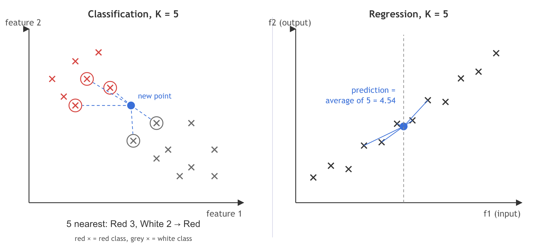
The video draws two groups of points: red ones and white ones. A new point lands between them. Logistic regression would draw a line; KNN asks a simpler question: what are the points closest to it?
With K = 5, KNN takes the 5 nearest training points. On the board, 3 of them are red and 2 are white. The majority is red, so the new point is classed red.
Measuring distance: Euclidean and Manhattan
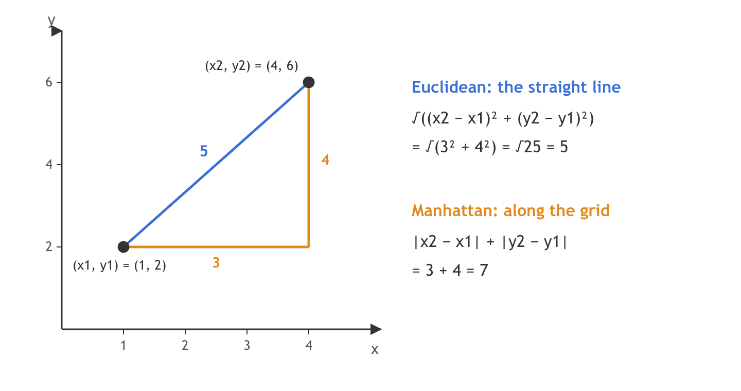
"Nearest" needs a distance. The video names two. For points (x1, y1) and (x2, y2), the Euclidean distance is the straight line between them, the hypotenuse of the right triangle:
The video reads this formula out without the square root; the distance needs it, as written above. The Manhattan distance walks along the two legs of the triangle instead of the hypotenuse, like a taxi on a grid of streets:
Predicting a number with KNN regression
For regression the output is a number. KNN finds the K = 5 nearest points in the same way, then predicts the average of their outputs. That is the only difference between the two uses, as the right panel of the diagram shows.
Choosing K by the error rate
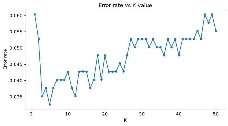
K is a hyperparameter: you choose it, the model does not learn it. The video's recipe is to try K = 1 to 50, measure the error rate for each one on data the model did not train on, and keep the K where the error rate is lowest.
Where KNN goes wrong: outliers and imbalanced data
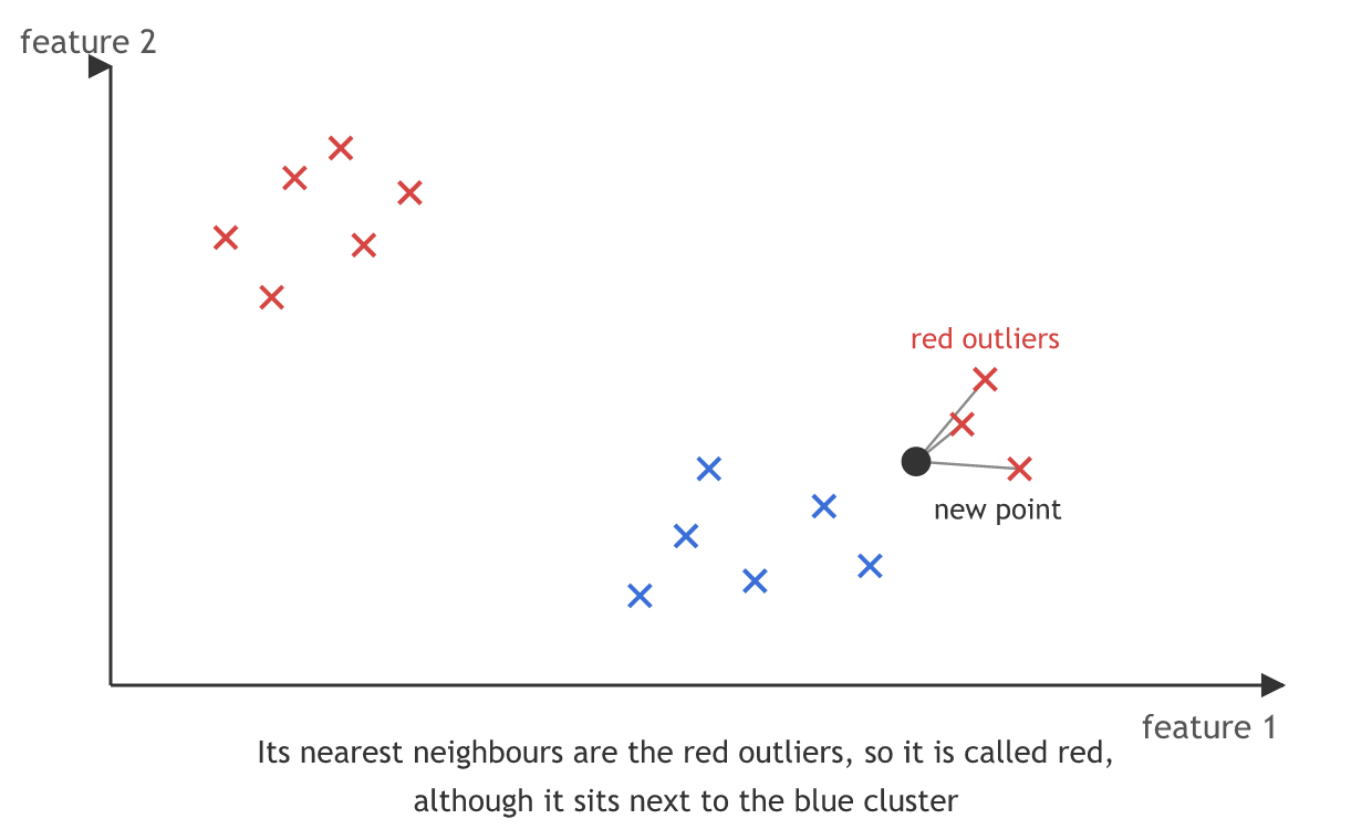
KNN works badly with two things. Outliers: a few red points far from the red group can sit right next to the blue group, and a new point there gets the red outliers as its nearest neighbours. Imbalanced data: if one class has far more points, it tends to win the vote by numbers alone.
Running KNN on the video's two groups
The points below copy the video's picture: a red group at the top left, a white group at the bottom right, and a new point between them.
Typing the two groups
# The video's picture: a red group at the top left, a white group at the bottom right
red = [(1, 7), (2, 8), (1.5, 6), (2.5, 7), (3, 8.5), (2, 5.5), (3.5, 6.5)]
white = [(6, 3), (7, 2), (5.5, 4.5), (8, 3), (7, 4.5), (5.5, 2.5), (8, 1.5), (6.5, 1.5), (4.5, 3.5)]
X = red + white
y = ["red"] * len(red) + ["white"] * len(white)
new_point = [[4.4, 5.5]]
Finding the five nearest neighbours
from sklearn.neighbors import KNeighborsClassifier

# K = 5, distance = Euclidean (the default metric, minkowski with p=2)
knn = KNeighborsClassifier(n_neighbors=5)
knn.fit(X, y)
distances, idx = knn.kneighbors(new_point) # the 5 closest training pointslabels = [y[i] for i in idx[0]]
print("5 nearest distances:", distances[0].round(2))
print("their classes: ", labels)
print("votes:", {c: labels.count(c) for c in sorted(set(labels))}, "->", knn.predict(new_point)[0])
# The same vote with Manhattan distance
manhattan = KNeighborsClassifier(n_neighbors=5, metric="manhattan").fit(X, y)
print("Manhattan ->", manhattan.predict(new_point)[0])
# Distances between (1, 2) and (4, 6)
from sklearn.metrics.pairwise import euclidean_distances, manhattan_distances
print(euclidean_distances([[1, 2]], [[4, 6]])[0][0], manhattan_distances([[1, 2]], [[4, 6]])[0][0])5 nearest distances: [1.35 1.49 2. 2.4 2.42]
their classes: ['red', 'white', 'white', 'red', 'red']
votes: {'red': 3, 'white': 2} -> red
Manhattan -> red
5.0 7.0What the five neighbours decide
- Three red, two white: the five nearest distances run from 1.35 to 2.42, and the vote is 3 to 2, so the new point is red, as on the board.
- Manhattan agrees here: changing the distance can change which points count as nearest, but for this point the vote is still red.
- 5.0 and 7.0: the straight-line and grid distances between (1, 2) and (4, 6), as in the distance diagram.
Choosing K on the breast cancer data
The video describes the K = 1 to 50 search without running it. Here it runs on scikit-learn's breast cancer dataset (569 tumours, 30 measurements each, labelled malignant or benign). Each K is scored with 5-fold Cross-validation on the training set, so the test set stays out of the choice and checks the chosen K once at the end. The features are put on the same scale first, for a reason the next section shows.
Scaling inside a pipeline
from sklearn.datasets import load_breast_cancer
from sklearn.model_selection import train_test_split, cross_val_score
from sklearn.pipeline import make_pipeline
from sklearn.preprocessing import StandardScaler

X, y = load_breast_cancer(return_X_y=True)
X_train, X_test, y_train, y_test = train_test_split(X, y, test_size=0.3, random_state=42, stratify=y)

def knn_model(k):
    # scale every feature to mean 0, std 1, then vote among k neighbours
return make_pipeline(StandardScaler(), KNeighborsClassifier(n_neighbors=k))import matplotlib.pyplot as plt
ks = range(1, 51)
# the error rate of each K from 5-fold cross-validation on the training set
error_rate = [1 - cross_val_score(knn_model(k), X_train, y_train, cv=5).mean() for k in ks]
best_k = min(ks, key=lambda k: error_rate[k - 1])
print("lowest error rate:", round(min(error_rate), 3), "at K =", best_k)
print("error rate at K = 1:", round(error_rate[0], 3))
test_acc = knn_model(best_k).fit(X_train, y_train).score(X_test, y_test)
print(f"test accuracy at K = {best_k}: {test_acc:.3f}")
plt.figure(figsize=(8, 4))
plt.plot(ks, error_rate, marker="o", markersize=4)
plt.title("Error rate vs K value")
plt.xlabel("K")
plt.ylabel("Error rate")
plt.show()lowest error rate: 0.033 at K = 5 error rate at K = 1: 0.06 test accuracy at K = 5: 0.959
Why KNN needs scaled features
Distances add up the differences in every feature. In the breast cancer data one feature (worst area) runs into the thousands while another (smoothness) stays below 0.2, so unscaled distance is almost all area. StandardScaler puts every feature on the same footing.
for name, model in [("no scaling  ", KNeighborsClassifier(n_neighbors=5)),
                    ("StandardScaler", knn_model(5))]:
    model.fit(X_train, y_train)
print(name, "test accuracy:", round(model.score(X_test, y_test), 3))no scaling test accuracy: 0.924 StandardScaler test accuracy: 0.959
What the error-rate search shows
- The lowest error rate is 0.033, at K = 5: that is the K the video's recipe keeps. K = 1 makes 0.06 errors, because a single neighbour follows every noisy point.
- Large K gets worse: past about K = 25 the error rate climbs back to around 0.05 and 0.06, because so many neighbours blur the border between the classes.
- The test set checks the choice once: K = 5 scores 0.959 on test data that played no part in choosing it. Picking K by the test score instead would make that score look better than it is.
- Scaling changes the answer: the same K = 5 model goes from 0.924 to 0.959 test accuracy once every feature is on the same scale.
Euclidean vs Manhattan distance
| Euclidean | Manhattan | |
|---|---|---|
| Path | Straight line (the hypotenuse) | Along the axes (the two legs) |
| Formula | √((x2 − x1)² + (y2 − y1)²) | |x2 − x1| + |y2 − y1| |
| (1, 2) to (4, 6) | 5 | 7 |
| In scikit-learn | metric="minkowski", p=2 (the default) | metric="manhattan" or p=1 |
| Effect of one big difference | Squared, so it dominates | Counted once, so it weighs less |
Where you use KNN
- Recommendations: "users like you" means users whose ratings are nearest to yours.
- Filling in missing values: scikit-learn's
KNNImputerfills a gap with the average of the nearest rows. - Small, low-dimensional data: a quick classifier with no training step, where you can see why each prediction was made.
Related
- Previous: Naive Bayes worked example
- Next: Decision tree classifier
- Reference: scikit-learn user guide, Nearest Neighbors
- Change
n_neighbors=5to 1 in the two-group example. Which single point decides, and does the class change? - Move the new point to
[[5.5, 4]]and run the vote again. - In the scaling example, swap
StandardScaler()forMinMaxScaler()(import it fromsklearn.preprocessing) and compare the accuracy.
Every expert started right here.