Entropy and Gini impurity
Entropy and Gini impurity are purity measures that score how mixed the classes in a decision tree node are: 0 for a pure node, and higher the more evenly the classes are mixed.
Last updated: 04 Oct, 2026 · scikit-learn 1.9.1
The Decision tree classifier split play tennis on Outlook and got one node with only Yes days and two mixed ones. To decide whether to split a node again, the tree needs a number for that mix.
Telling a pure split from an impure split
Look again at the three Outlook nodes. Overcast is 4 Yes and 0 No. Every Overcast day is a Yes, so if day 15 is Overcast, the answer is Yes without asking anything else. A node whose records all have one class is pure; it becomes a pure leaf node and is not split again.
Sunny is 2 Yes and 3 No, and Rain is 3 Yes and 2 No. Mixed nodes are impure. The tree takes another feature (Temperature, say, under Sunny) and keeps splitting until it reaches pure leaves.
That leaves two questions. How do we measure purity? With entropy or Gini impurity, both covered here. Which feature do we split on? With information gain, covered in Information gain. The board writes "Gini coefficient"; the right name, as the video says, is Gini impurity.
Computing entropy for a pure node
For two classes, write p₊ for the probability of Yes in the node and p₋ for the probability of No. The entropy of the sample S is:
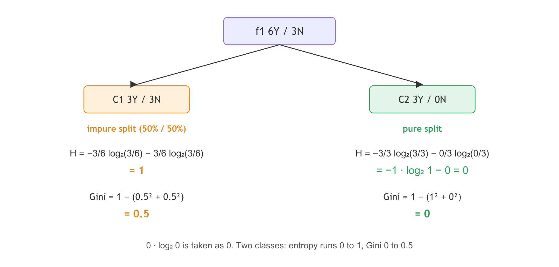
The video's example: a feature f1 at the root holds 6 Yes and 3 No. It has two categories, so it splits into C1 with 3 Yes and 3 No and C2 with 3 Yes and 0 No. The children add back up: 3 + 3 = 6 Yes and 3 + 0 = 3 No.
For C2, p₊ = 3/3 = 1 and p₋ = 0/3 = 0:
log₂ 0 itself is undefined; the term 0 · log₂ 0 is taken as 0, because p · log₂ p shrinks to 0 as p does. So a pure split always has entropy 0.
Reading the entropy curve
Now C1, with 3 Yes and 3 No. Here p₊ = 3/6 = 0.5 and p₋ = 0.5 (since p₋ = 1 − p₊):
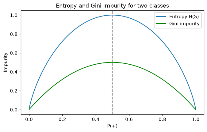
Plot H(S) against p₊ and you get the board's curve. It is 0 at p₊ = 0 and at p₊ = 1 (pure nodes), and it peaks at 1 when p₊ = 0.5, the most mixed a two-class node can be. For two classes, entropy always lies between 0 and 1. For any other mix you read the value off the curve: at p₊ = 0.3 it is about 0.88.
Computing Gini impurity
Gini impurity adds up the squared class probabilities and subtracts them from 1. With n output classes:
The video's example is a node with 2 Yes and 2 No, so p₊ = p₋ = 1/2:
The same node has entropy 1. So for two classes, Gini impurity runs from 0 (pure) to 0.5 (a 50/50 mix), and its curve sits under the entropy curve, peaking at 0.5 at p₊ = 0.5.
Both measures work for more than two classes. Gini impurity already sums over all n classes. Entropy adds one term per class, so for an output with three categories c₁, c₂ and c₃ it reads:
Choosing between Gini and entropy
The difference is speed. Entropy needs a logarithm; Gini needs only squares. A tree computes impurity again and again, for every candidate split of every feature, so with many features (100 or 200) the cheaper formula adds up. The video's advice: with many features use Gini impurity, with a small set entropy is fine. scikit-learn's DecisionTreeClassifier uses Gini by default.
The number of records points the same way. Every record adds candidate splits to score, so a small dataset can afford entropy, and a large one is a reason to prefer Gini impurity.
The board writes "Gini >> Entropy" for speed; Gini is faster, but by a modest margin, and the two measures often choose the same splits.
Computing entropy and Gini in Python
An entropy function
import numpy as np

def entropy(counts):
    p = np.array(counts) / sum(counts)
    p = p[p > 0]                      # 0 * log2(0) counts as 0
    return float((p * np.log2(1 / p)).sum())   # same as -sum(p * log2(p))
A Gini impurity function
def gini(counts):
    p = np.array(counts) / sum(counts)
return float(1 - (p ** 2).sum())nodes = {"f1 root 6Y/3N": [6, 3], "C1 3Y/3N": [3, 3], "C2 3Y/0N": [3, 0],
"2Y/2N": [2, 2], "p+ = 0.3": [3, 7], "play tennis 9Y/5N": [9, 5],
"three equal classes": [1, 1, 1]}
for name, counts in nodes.items():
print(f"{name:20} entropy {entropy(counts):.3f} gini {gini(counts):.3f}")f1 root 6Y/3N entropy 0.918 gini 0.444 C1 3Y/3N entropy 1.000 gini 0.500 C2 3Y/0N entropy 0.000 gini 0.000 2Y/2N entropy 1.000 gini 0.500 p+ = 0.3 entropy 0.881 gini 0.420 play tennis 9Y/5N entropy 0.940 gini 0.459 three equal classes entropy 1.585 gini 0.667
Plotting the entropy and Gini curves
import numpy as np
import matplotlib.pyplot as plt

p = np.linspace(0.001, 0.999, 300)                   # P(+), the share of Yes
H = -p * np.log2(p) - (1 - p) * np.log2(1 - p)       # entropy
G = 1 - p ** 2 - (1 - p) ** 2                        # Gini impurity

plt.figure(figsize=(7, 4))
plt.plot(p, H, label="Entropy H(S)")
plt.plot(p, G, label="Gini impurity", color="green")
plt.axvline(0.5, linestyle="--", color="grey")
plt.title("Entropy and Gini impurity for two classes")
plt.xlabel("P(+)")
plt.ylabel("Impurity")
plt.legend()
plt.show()
print("peak entropy:", round(H.max(), 3), " peak gini:", round(G.max(), 3))peak entropy: 1.0 peak gini: 0.5
What the impurity values show
- C2 3Y/0N gives 0 and 0: a pure node has no impurity on either measure.
- C1 3Y/3N gives entropy 1 and Gini 0.5: the two-class maximums, as on the board.
- The root 6Y/3N gives 0.918 and 0.444: a mix between pure and 50/50. Play tennis's 9Y/5N gives 0.940, the 0.94 used in the information gain lesson.
- p₊ = 0.3 gives entropy 0.881: the value read off the curve.
- Three equal classes give entropy 1.585 and Gini 0.667: with more classes both maximums grow. The 0 to 1 and 0 to 0.5 ranges hold for two classes only.
Entropy vs Gini impurity
| Entropy | Gini impurity | |
|---|---|---|
| Formula | −Σ pᵢ log₂ pᵢ | 1 − Σ pᵢ² |
| Pure node | 0 | 0 |
| 50/50, two classes | 1 | 0.5 |
| Three equal classes | log₂ 3 = 1.585 | 1 − 3 × (1/3)² = 0.667 |
| Cost | Needs a logarithm | Only squares, a little faster |
| In DecisionTreeClassifier | criterion="entropy" or "log_loss" | criterion="gini" (the default) |
Where you use entropy and Gini impurity
- Choosing the criterion:
DecisionTreeClassifier(criterion="gini")orcriterion="entropy"; in scikit-learn, "entropy" and "log_loss" both mean the Shannon entropy. - Reading a fitted tree:
plot_treeprints the Gini value of every node, so you can see where the tree is still unsure. - Scoring a split: information gain subtracts the children's entropy from the parent's.
Related
- Previous: Decision tree classifier
- Next: Information gain
- Reference: scikit-learn user guide, classification criteria
- Add
"Sunny 2Y/3N": [2, 3]to the nodes and compare it with Rain's[3, 2]. Why are they equal? - Try four equal classes,
[1, 1, 1, 1]. Is the Gini value 1 − 4 × (1/4)² = 0.75? - Mark p₊ = 0.3 on the plot with
plt.scatter([0.3], [0.881], color="red")beforeplt.show().
You understood something today that you didn't yesterday.