Decision tree regression and pruning
A decision tree regressor is a decision tree that predicts a number: each leaf outputs the mean of its training targets, and the splits are chosen to lower the mean squared error.
Last updated: 04 Oct, 2026 · scikit-learn 1.9.1
The trees in Information gain predicted a class. When the output is continuous, such as a price or a score, the same tree works with two changes: a leaf gives an average, and the purity test becomes the squared error.
The video calls the criteria mean squared error and mean absolute error. scikit-learn names them "squared_error" and "absolute_error"; the older names "mse" and "mae" were removed in version 1.2.
Predicting the mean in each node
Say feature f1 is chosen for the root. The root's prediction is the mean of all the outputs. Instead of entropy or Gini, the tree measures how far the outputs are from that mean with the mean squared error (MSE), or the mean absolute error (MAE):
The board borrows 1/2m from the linear regression cost function; the MSE of a node divides by n, the number of records in it.
Then the tree splits. Some records go to one child, the rest to the other, and each child predicts the mean of its own records. A good split makes the MSE drop. Following a path down to a leaf, the output is the mean of the records in that leaf.
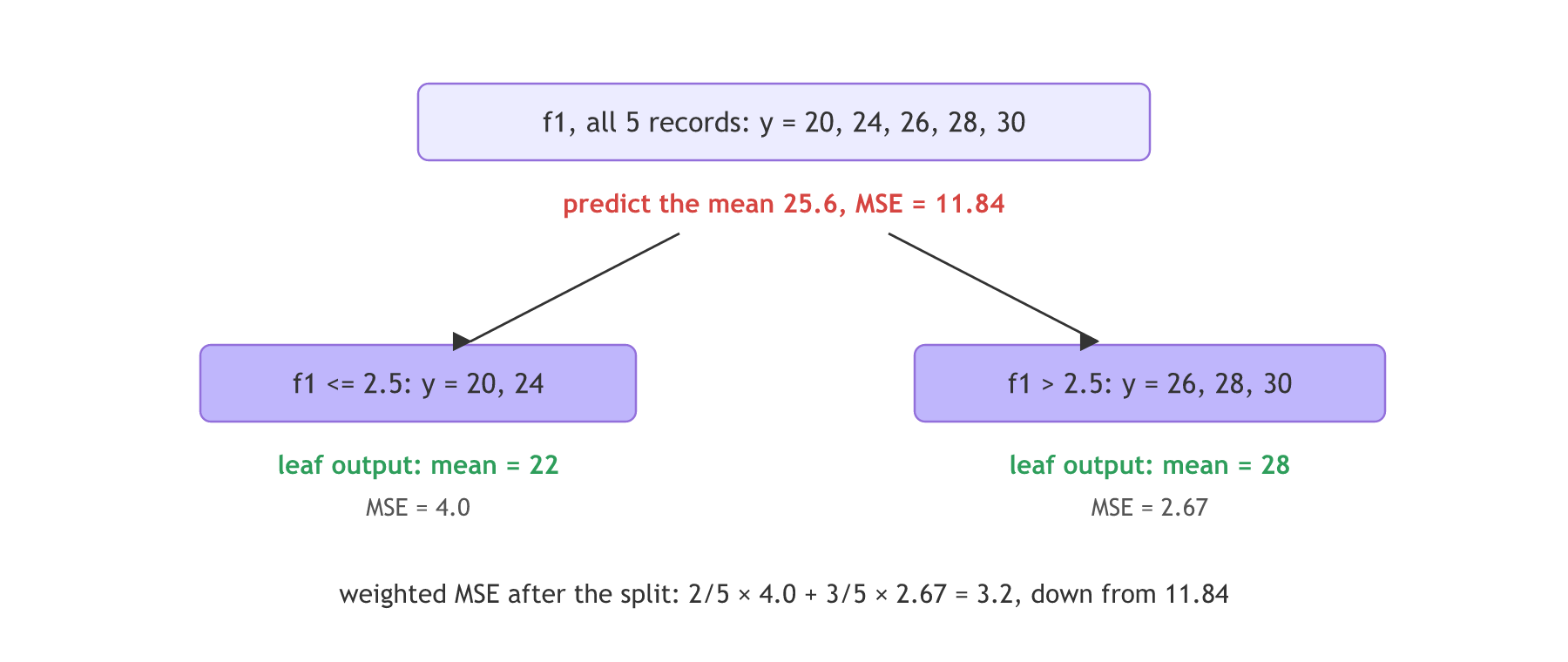
The video's example has five outputs: 20, 24, 26, 28 and 30. Their mean is 25.6, so the root predicts 25.6, and its MSE is
The clip calls the MSE "some 37, 47" as a stand-in number; for these five values it is 11.84. If the first two records go left and the other three right, the left leaf predicts 22 with MSE 4, the right leaf predicts 28 with MSE 2.67, and the weighted MSE falls to 3.2.
Scoring a split with variance reduction
The MSE of a node around its own mean is the variance of its outputs. So the drop in MSE that a split buys has a name: variance reduction. A regression tree tries every candidate split and keeps the one with the largest variance reduction, the way a classification tree keeps the largest information gain. For the five targets above it is 11.84 − 3.2 = 8.64.
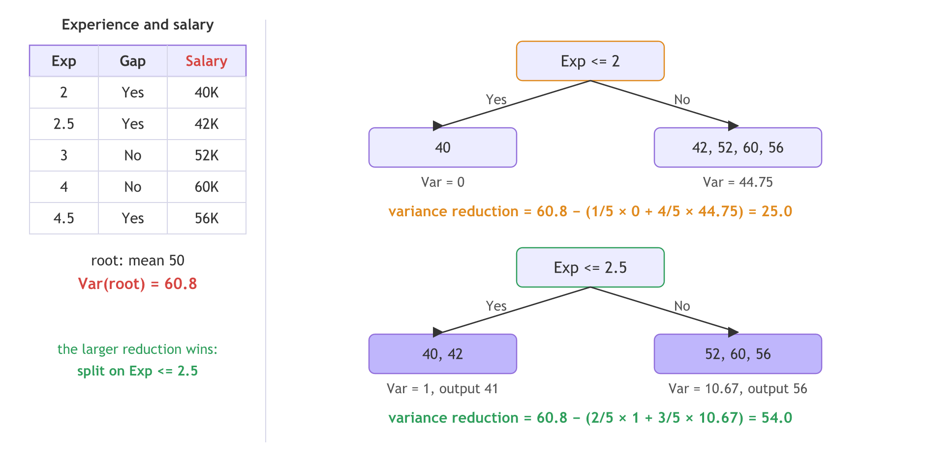
A second example makes the search visible. Five people have years of experience, a career gap (Yes or No) and a salary, the output:
| Exp | Gap | Salary |
|---|---|---|
| 2 | Yes | 40K |
| 2.5 | Yes | 42K |
| 3 | No | 52K |
| 4 | No | 60K |
| 4.5 | Yes | 56K |
The mean salary is 50K, so the root predicts 50 and its variance is:
Now try two thresholds on Exp. Each child's variance is weighted by its share of the records wᵢ and subtracted from the root's:
- Exp ≤ 2 leaves 40 alone (variance 0) and 42, 52, 60, 56 on the other side (mean 52.5, variance 44.75). The reduction is 60.8 − (1/5 × 0 + 4/5 × 44.75) = 25.0.
- Exp ≤ 2.5 leaves 40, 42 (mean 41, variance 1) and 52, 60, 56 (mean 56, variance 10.67). The reduction is 60.8 − (2/5 × 1 + 3/5 × 10.67) = 54.0, the larger one, so the tree splits here.
A new person who lands in the left leaf gets the mean of 40 and 42, a salary of 41K; one in the right leaf gets (52 + 60 + 56) / 3 = 56K. A common slip is to measure each child's spread from the root's mean of 50, which gives reductions of 0 and 0.004; each child's variance is measured from its own mean, which gives 25.0 and 54.0. The winner, Exp ≤ 2.5, is the same either way.
Pruning a tree that overfits
A decision tree can keep dividing nodes to any depth, so it tends to overfit: it learns the training data, noise included. Cutting the tree back is called pruning, and there are two kinds.
Post-pruning builds the full tree first, then looks for branches that add little. The video's example is a node with 7 Yes and 2 No. Most of its records, 7 of 9 or about 78%, are Yes, so splitting it further adds little: cut the branch and let the node answer Yes.
Pre-pruning stops the tree while it grows, with hyperparameters such as max_depth (how many questions deep) and max_leaf_nodes (how many leaves at most). Their values are tuned with GridSearchCV, as in Hyperparameter tuning with GridSearchCV.
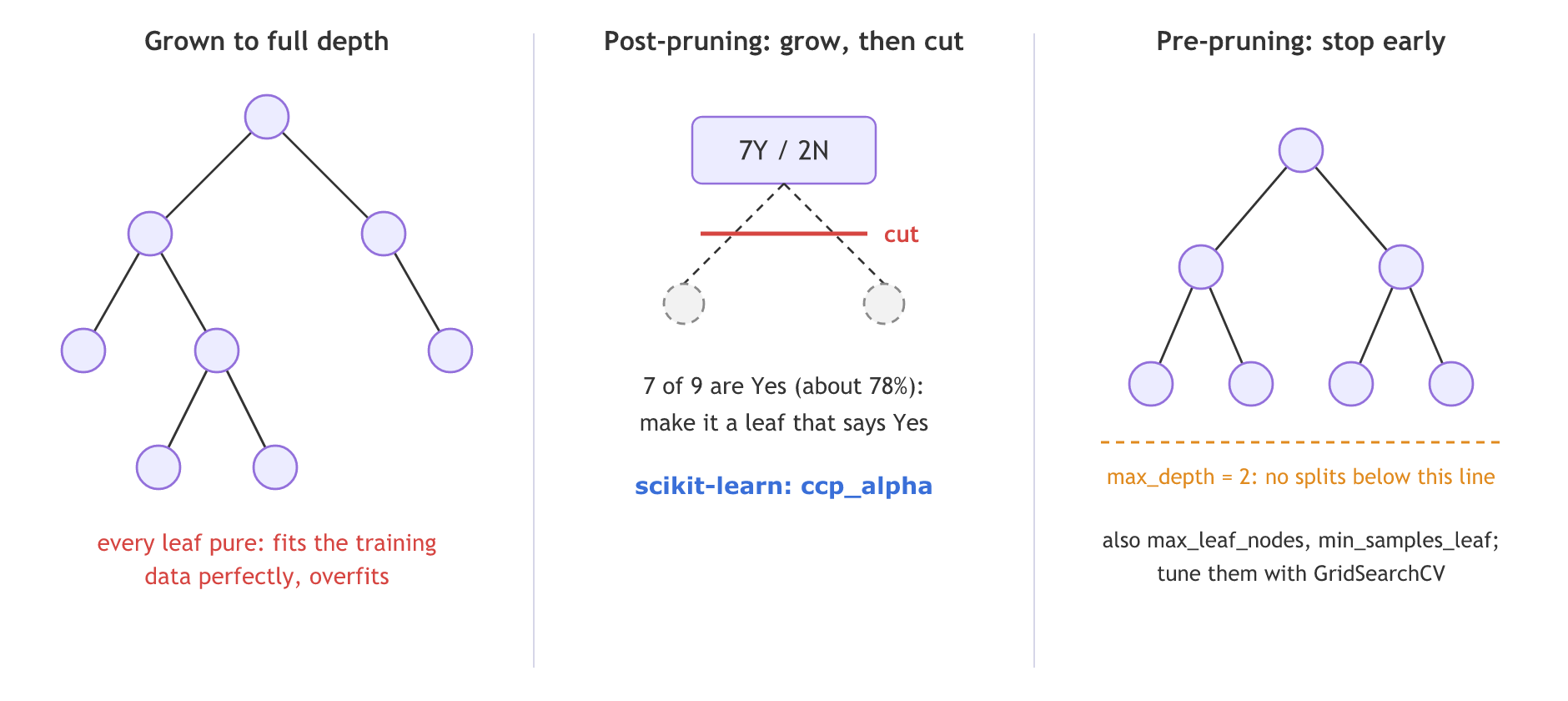
The video describes post-pruning without code. In scikit-learn it is minimal cost-complexity pruning, set with ccp_alpha. Each subtree T is scored by its error R(T) plus a charge of α for every leaf, and the tree keeps the subtree with the lowest score. A bigger α means a smaller tree.
Fitting the five targets with DecisionTreeRegressor
The five records
import numpy as np
from sklearn.tree import DecisionTreeRegressor, export_text

# One feature f1 and the five continuous targets from the video
f1 = np.array([[1], [2], [3], [4], [5]])
y = np.array([20, 24, 26, 28, 30])
Using the old criterion name
Code written for older releases passes criterion="mse". On scikit-learn 1.9.1 it fails before fitting:
try:
    DecisionTreeRegressor(criterion="mse").fit(f1, y)
except ValueError as err:
    print(type(err).__name__)
print(str(err).split(" among")[0]) # the message goes on to list the accepted namesInvalidParameterError The 'criterion' parameter of DecisionTreeRegressor must be a str
print("root: mean", y.mean(), "MSE", round(((y - y.mean()) ** 2).mean(), 2))

reg = DecisionTreeRegressor(criterion="squared_error", max_depth=1).fit(f1, y)
print(export_text(reg, feature_names=["f1"]))
print("node MSEs:", reg.tree_.impurity.round(2))
print("predictions for f1 = 2 and 4:", reg.predict([[2], [4]]))root: mean 25.6 MSE 11.84 |--- f1 <= 2.50 | |--- value: [22.00] |--- f1 > 2.50 | |--- value: [28.00] node MSEs: [11.84 4. 2.67] predictions for f1 = 2 and 4: [22. 28.]
What the regressor found
- Root mean 25.6, MSE 11.84: the numbers worked out above.
- The split is f1 ≤ 2.5: of all the places to cut, putting 20 and 24 on one side and 26, 28, 30 on the other lowers the MSE the most.
- Node MSEs 11.84, 4.0 and 2.67: the root, then the two leaves. Each leaf predicts its mean, 22 or 28.
- "mse" is rejected with an
InvalidParameterError, a kind ofValueError. The full message goes on to list the names 1.9.1 accepts:"squared_error","absolute_error"and"poisson".
Computing variance reduction for the salary data
The salary records
import numpy as np
from sklearn.tree import DecisionTreeRegressor

# Years of experience and salary in thousands
exp = np.array([[2], [2.5], [3], [4], [4.5]])
salary = np.array([40, 42, 52, 60, 56])for i, cut in enumerate(exp[:-1, 0]):
left, right = salary[: i + 1], salary[i + 1:]
weighted = len(left) / 5 * left.var() + len(right) / 5 * right.var()
print(f"Exp <= {cut}: variance reduction {salary.var() - weighted:.1f}")
stump = DecisionTreeRegressor(max_depth=1).fit(exp, salary)
print("scikit-learn threshold:", round(stump.tree_.threshold[0], 2))
print("predictions for Exp = 2.2 and 4.2:", stump.predict([[2.2], [4.2]]))Exp <= 2.0: variance reduction 25.0 Exp <= 2.5: variance reduction 54.0 Exp <= 3.0: variance reduction 42.7 Exp <= 4.0: variance reduction 9.0 scikit-learn threshold: 2.75 predictions for Exp = 2.2 and 4.2: [41. 56.]
var() on a NumPy array divides by n, the same variance as the formula. The loop finds 25.0 for Exp ≤ 2 and 54.0 for Exp ≤ 2.5, the two splits worked out above, and scikit-learn picks the same split. It places the threshold at 2.75, halfway between 2.5 and 3, and the two leaves predict 41 and 56.
Pre-pruning and post-pruning on the diabetes data
Pruning pays off on real data. scikit-learn's diabetes dataset has 442 patients with ten measurements each (age, sex, BMI, blood pressure and six blood serum values, already centred and scaled). The output is a number: how far the disease progressed one year later. The data is split 70/30, and three regression trees are compared: no limits, pre-pruned with GridSearchCV, and post-pruned with ccp_alpha.
Loading and splitting the diabetes data
import numpy as np
from sklearn.tree import DecisionTreeRegressor
from sklearn.datasets import load_diabetes
from sklearn.model_selection import train_test_split, GridSearchCV, cross_val_score
from sklearn.metrics import r2_score, mean_squared_error

X, y = load_diabetes(return_X_y=True, as_frame=True)   # 442 patients, 10 features
X_train, X_test, y_train, y_test = train_test_split(X, y, test_size=0.3, random_state=10)
Pre-pruning with GridSearchCV
The grid tries the criterion, the splitter, the depth and how many features each split may look at. neg_mean_squared_error is the MSE with its sign flipped, because GridSearchCV keeps the highest score. Older code for this search also lists criterion="friedman_mse" and max_features="auto"; scikit-learn 1.9.1 rejects both for DecisionTreeRegressor ("auto" was removed in 1.3), so None, meaning all features, takes the place of "auto".
# Pre-pruning: search the limits with 5-fold cross-validation
param = {
    "criterion": ["squared_error", "absolute_error"],
    "splitter": ["best", "random"],
    "max_depth": [1, 2, 3, 4, 5, 10, 15, 20, 25],
    "max_features": [None, "sqrt", "log2"],
}
grid = GridSearchCV(DecisionTreeRegressor(random_state=42), param_grid=param,
                    cv=5, scoring="neg_mean_squared_error")
grid.fit(X_train, y_train)
Post-pruning with ccp_alpha
# Post-pruning: grow the full tree, list the alphas at which branches get cut,
# then keep the alpha with the best 5-fold cross-validation score
path = DecisionTreeRegressor(random_state=42).cost_complexity_pruning_path(X_train, y_train)
alphas = path.ccp_alphas[:-1]        # the last alpha cuts the tree down to its root
cv = [cross_val_score(DecisionTreeRegressor(ccp_alpha=a, random_state=42), X_train, y_train,
                      cv=5, scoring="neg_mean_squared_error").mean() for a in alphas]
best_alpha = alphas[int(np.argmax(cv))]
pruned = DecisionTreeRegressor(ccp_alpha=best_alpha, random_state=42).fit(X_train, y_train)print("best grid:", grid.best_params_)
print("best ccp_alpha:", round(best_alpha, 1))
full = DecisionTreeRegressor(random_state=42).fit(X_train, y_train)
for name, model in [("no limits", full), ("grid search", grid.best_estimator_), ("ccp_alpha", pruned)]:
pred = model.predict(X_test)
print(f"{name:12} depth {model.get_depth():2} leaves {model.get_n_leaves():3} "
f"train R2 {model.score(X_train, y_train):.3f} test R2 {r2_score(y_test, pred):.3f} "
f"test MSE {mean_squared_error(y_test, pred):.0f}")best grid: {'criterion': 'squared_error', 'max_depth': 4, 'max_features': None, 'splitter': 'random'}
best ccp_alpha: 126.4
no limits depth 19 leaves 302 train R2 1.000 test R2 -0.191 test MSE 7534
grid search depth 4 leaves 13 train R2 0.408 test R2 0.248 test MSE 4758
ccp_alpha depth 5 leaves 7 train R2 0.506 test R2 0.324 test MSE 4277What pruning changed
- The tree with no limits has 302 leaves for 309 training patients and a training R² of 1.000, but a test R² of −0.191. A negative R² means it does worse than predicting the average progression for every patient: it memorised the training rows.
- The grid search keeps depth 4 and 13 leaves (squared error, random splitter, all features) and lifts the test R² to 0.248, with the test MSE down from 7534 to 4758.
- Cost-complexity pruning keeps 7 leaves with ccp_alpha 126.4 and gives the best test score here, R² 0.324 and MSE 4277, with the smallest tree.
- The training R² drops for both pruned trees, to 0.408 and 0.506. That is the point: they stop memorising the training rows. An R² near 0.3 also shows that one tree is a weak model for this data; the ensembles in Bagging and boosting combine many trees to do better.
Pre-pruning vs post-pruning
| Pre-pruning | Post-pruning | |
|---|---|---|
| When | While the tree grows | After the full tree is built |
| How | Limits on depth, leaves or samples per leaf | Cut weak branches, like the 7Y/2N node |
| In scikit-learn | max_depth, max_leaf_nodes, min_samples_leaf | ccp_alpha (minimal cost-complexity pruning) |
| Tuning | GridSearchCV over the limits | cost_complexity_pruning_path, then cross-validation |
| On the diabetes data | depth 4, 13 leaves, test R² 0.248 | 7 leaves, test R² 0.324 |
| Cost | Cheap: the tree stays small | Grows the full tree first |
Where you use decision tree regression
- Prices and amounts with thresholds: rent by area and number of rooms, where the effect jumps at certain values.
- A quick non-linear baseline: no scaling, no assumption of a straight-line relationship.
- Inside ensembles: random forest and gradient boosting regressors are many regression trees added together.
Related
- Previous: Information gain
- Next: Decision tree in scikit-learn
- Reference: scikit-learn user guide, minimal cost-complexity pruning
- Predict
reg.predict([[10]])and confirm the answer is 28. - Set
max_depth=2on the five-record regressor. How many leaves are there, and what are their means? - Change the regressor to
criterion="absolute_error"and print the tree again. Each leaf now predicts the median of its records. Does the split stay at f1 ≤ 2.5?
This is what real progress feels like.