Ridge regression
Ridge regression is a linear regression that adds λ times the sum of the squared slopes to the cost function, so the fitted line cannot become steep enough to overfit.
Last updated: 05 Oct, 2026 · scikit-learn 1.9.1
The two-point line in Overfitting and underfitting had a cost of 0 and still failed on new points. Ridge changes the cost so that a zero error alone no longer wins.
The board first writes 0 + 1(2) = 3, then corrects it to 0 + 1 × 2² = 4.
Adding a penalty to the cost function
Back to the two points. The cost is 1/2m Σ (hθ(x(i)) − y(i))²; writing hθ(x) as ŷ, each term is (ŷ(i) − y(i))², the difference between the predicted and the real value. Here every difference is 0, so the cost is 0, "and this is still overfitting".
Ridge, also called L2 regularization, adds one more term to the cost: λ multiplied by the slope squared. With the line through the origin θ₀ = 0, so hθ(x) = θ₁x and θ₁ is the slope.
The video's numbers: λ = 1 and a slope of 2, the slope of the line through both points. The error is 0 and the penalty is 1 × 2² = 4, so the cost is 4, not 0. Gradient descent keeps going: it changes θ₁ to bring the 4 down.
Trading a small error for a flatter line
Changing θ₁ gives the next best fit line, a less steep one. The video takes a slope of 1.5. This line no longer passes through the points, so the error becomes a small value, and the penalty is 1 × 1.5² = 2.25. The cost is that small value plus 2.25, which the video puts at about 3. It is less than 4, so Ridge prefers the flatter line.
The lesson of the picture: "the slope should not be steep". A steep slope most of the time leads to overfitting. New points land closer to the flatter line, so it generalizes better, low bias and low variance instead of the overfit condition.
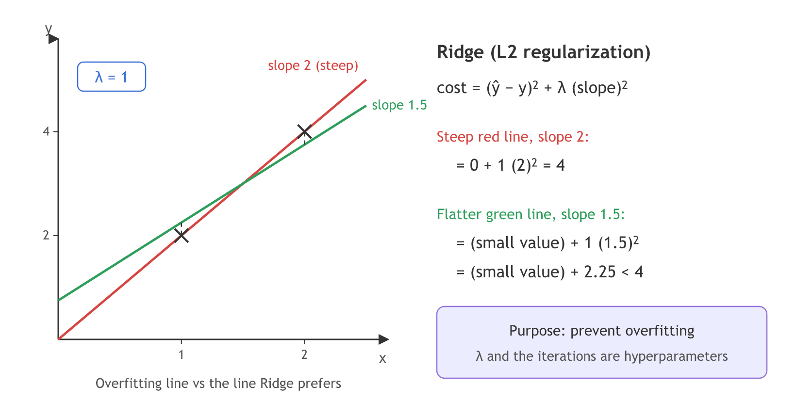
λ is a hyperparameter: a value you choose, not one the model learns. It sets how hard the steepness is pushed down. The number of iterations, how many times θ₁ is updated, is a hyperparameter too. The Hyperparameter tuning with GridSearchCV lesson chooses λ by search.
Checking the video's numbers in code
The board does not give the two points, only the slope of 2. Any two points on the line y = 2x work; the code takes (1, 2) and (2, 4) and adds up the error and the penalty the way the board does, with λ = 1.
The Ridge class
scikit-learn calls λ alpha. Ridge minimises ‖y − Xw‖² + alpha ‖w‖²: the sum of the squared errors plus alpha times the sum of the squared slopes, with no 1/2m in front, the form Σ(ŷ − y)² + λ slope² the board uses for its numbers. fit_intercept=False keeps θ₀ = 0, as in the video.
from sklearn.linear_model import Ridge

# alpha is the λ of the board; fit_intercept=False keeps θ0 = 0
ridge = Ridge(alpha=1, fit_intercept=False)
ridge.fit(X, y)          # X has one column per feature
print(ridge.coef_)       # the slopes after the penalty
Scoring slope 2, slope 1.5 and the Ridge slope
import numpy as np
from sklearn.linear_model import Ridge

x = np.array([1.0, 2.0])
y = np.array([2.0, 4.0])      # two points on the line y = 2x
lam = 1

def ridge_cost(slope):
    error = np.sum((slope * x - y) ** 2)   # sum of (y_hat - y)^2
    penalty = lam * slope ** 2             # lambda * slope^2
    return error, penalty, error + penalty

for slope in [2, 1.5]:
    error, penalty, cost = ridge_cost(slope)
    print(f"slope {slope}: error {error:.2f} + penalty {penalty:.2f} = cost {cost:.2f}")

ridge = Ridge(alpha=lam, fit_intercept=False).fit(x.reshape(-1, 1), y)
best = ridge.coef_[0]
error, penalty, cost = ridge_cost(best)
print(f"Ridge slope {best:.3f}: error {error:.3f} + penalty {penalty:.3f} = cost {cost:.3f}")slope 2: error 0.00 + penalty 4.00 = cost 4.00 slope 1.5: error 1.25 + penalty 2.25 = cost 3.50 Ridge slope 1.667: error 0.556 + penalty 2.778 = cost 3.333
Reading the Ridge slope
- Slope 2 costs 4.00. No error, all penalty: the board's 0 + 1 × 2² = 4.
- Slope 1.5 costs 3.50. For these two points the "small value" is 1.25, so the board's "about 3" is 3.5 here. It is below 4, as the video says.
- Ridge finds slope 1.667 with cost 3.333. That is the lowest cost of all slopes: Ridge gives up a small error (0.556) to cut the penalty. Neither line from the board is the exact minimum; the minimum sits between them.
- The slope that fits the points exactly no longer wins. Once λ is above 0, a perfect fit on the training data is not the cheapest answer.
Moving the lowest cost with λ
The cost can be drawn as a curve over every slope θ₁, the bowl that gradient descent walks down. With λ = 0 it is the plain squared error, and its lowest point, the global minimum, sits at slope 2: the overfit line. Adding λθ₁² lifts the curve more the farther θ₁ is from 0, so as λ grows the bowl rises and its lowest point slides toward 0: λ up, slope down. For the two points the lowest point has a short formula, θ₁ = 10 / (5 + λ).
import numpy as np
import matplotlib.pyplot as plt
from sklearn.linear_model import Ridge

x = np.array([1.0, 2.0])
y = np.array([2.0, 4.0])
theta1 = np.linspace(-0.2, 2.4, 261)              # the slopes to try

for lam, color in [(0, "black"), (10, "orangered"), (30, "goldenrod")]:
    cost = np.array([np.sum((t * x - y) ** 2) + lam * t ** 2 for t in theta1])
    ridge = Ridge(alpha=lam, fit_intercept=False).fit(x.reshape(-1, 1), y)
    print(f"lambda {lam:2}: lowest cost at slope {theta1[cost.argmin()]:.2f}, Ridge slope {ridge.coef_[0]:.3f}")
    plt.plot(theta1, cost, color=color, label=f"lambda = {lam}")

plt.title("Ridge cost for three values of lambda")
plt.xlabel("slope theta1")
plt.ylabel("J(theta1)")
plt.legend()
plt.show()lambda 0: lowest cost at slope 2.00, Ridge slope 2.000 lambda 10: lowest cost at slope 0.67, Ridge slope 0.667 lambda 30: lowest cost at slope 0.29, Ridge slope 0.286
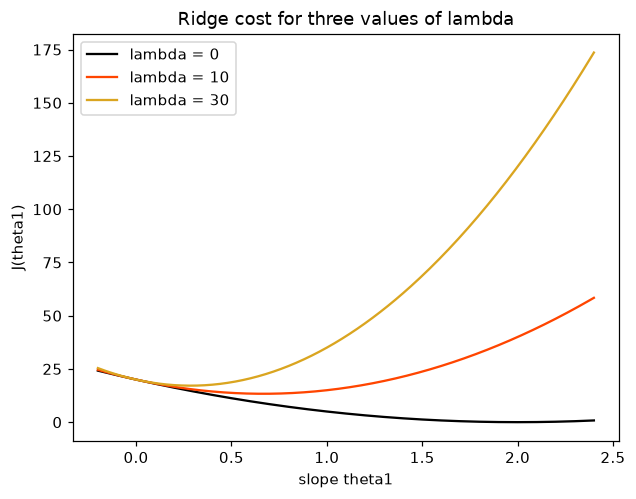
What the three curves show
- λ = 0 keeps the overfit line. The lowest cost is at slope 2, where the line passes through both points.
- λ = 10 moves it to 0.667 and λ = 30 to 0.286. The search over the curve and scikit-learn's Ridge agree, and both match 10 / (5 + λ).
- The slope never reaches 0. 10 / (5 + λ) stays above 0 for every λ, so Ridge flattens the line without removing the feature.
Shrinking coefficients on California housing
With many features, every slope gets the same treatment. A fitted line ŷ = 0.34 + 0.52x₁ + 0.48x₂ + 0.24x₃ might become ŷ = 0.34 + 0.40x₁ + 0.38x₂ + 0.14x₃ under Ridge: every slope smaller, none of them 0, and the intercept left alone. The California housing data shows it for real. It has 20,640 districts, 8 features (median income MedInc, house age, average rooms, average bedrooms, population, average occupancy, latitude, longitude) and the median house value as the target. StandardScaler first rescales each feature to mean 0 and standard deviation 1, so that one alpha pushes on every slope equally.
import pandas as pd
from sklearn.datasets import fetch_california_housing
from sklearn.preprocessing import StandardScaler
from sklearn.linear_model import Ridge

data = fetch_california_housing(as_frame=True)
X = StandardScaler().fit_transform(data.data)
y = data.target

coefs = {}
for alpha in [1, 100, 1000, 10000]:
    coefs[f"alpha={alpha}"] = Ridge(alpha=alpha).fit(X, y).coef_
table = pd.DataFrame(coefs, index=data.feature_names).round(3)
print(table)
print("sum of |coef|:", table.abs().sum().round(2).tolist())alpha=1 alpha=100 alpha=1000 alpha=10000 MedInc 0.830 0.826 0.782 0.526 HouseAge 0.119 0.125 0.151 0.120 AveRooms -0.265 -0.252 -0.150 0.035 AveBedrms 0.306 0.289 0.171 -0.019 Population -0.004 -0.002 0.007 0.001 AveOccup -0.039 -0.040 -0.040 -0.026 Latitude -0.899 -0.843 -0.553 -0.162 Longitude -0.870 -0.813 -0.518 -0.122 sum of |coef|: [3.33, 3.19, 2.37, 1.01]
What a larger alpha does to the slopes
- The slopes shrink toward 0. The sum of the absolute coefficients falls from 3.33 at alpha 1 to 1.01 at alpha 10000.
- None of them becomes exactly 0. Squaring makes the penalty on a small slope tiny, so Ridge never removes a feature. Population ends at 0.001, small but not zero.
- alpha 1 and alpha 100 are almost the same. scikit-learn's Ridge adds the penalty to a sum of squared errors over 20,640 rows, so alpha has to be large before it matters on a big data set.
- Strongly linked features move together. Latitude and Longitude shrink from −0.899 and −0.870 to −0.162 and −0.122 at the same pace, and AveRooms changes sign: with a heavy penalty, Ridge spreads the weight across features that carry the same information.
Ridge vs linear regression
| Linear regression | Ridge regression | |
|---|---|---|
| Cost | squared error | squared error + λ Σ θⱼ² |
| Two-point line | slope 2, cost 0 | slope 1.667 with λ = 1 |
| Coefficients | whatever fits the training data best | pulled toward 0, never exactly 0 |
| Extra setting | none | alpha (λ), chosen by cross-validation |
| alpha = 0 | the same as linear regression |
Where you use Ridge regression
- An overfit linear model. When the training score is much higher than the test score, a Ridge penalty is the first thing to try.
- Many polynomial or one-hot features. Like the degree 15 model in Overfitting and underfitting, where the slopes grow huge without a penalty.
- Correlated features. When two features carry the same information (multicollinearity, in Linear regression assumptions), Ridge keeps their slopes small and steady.
Related
- Previous: Bias and variance
- Next: Lasso regression
- Reference: scikit-learn: Ridge regression
- Set
lam = 0in the first example. The penalty disappears and slope 2 becomes the cheapest line again. - Change
lamto 0.25. The Ridge slope works out to 10 / (5 + 0.25) = 1.905, closer to 2. - Add
100000to the alpha list in the California run and see how close to 0 every slope gets.
You understood something today that you didn't yesterday.